Variance Explained and Variance Partitioning
As mentioned in Centroids and Inertia, The
"inertia" in a data set is analogous to the variance. For linear
methods, the inertia represents the variance in species abundance
(or transformed species abundance), but in unimodal methods, it represents
the variance or spread of species scores.
The following example is from a data set of vegetation (including forested
and nonforested areas, wet and dry grasslands, and varying bedrock type)
of the Nature Conservancy's Tallgrass Prairie Preserve in Osage County,
Oklahoma. The cover of vascular plants was estimated in a number
of 10m x 10m quadrats, and a number of environmental variables were measured,
including topographic information, woody cover, and soil data.
An excerpt of the output (*.log file) of a CCA follows:
N name (weighted)
mean stand. dev. inflation factor
1 SPEC AX1
.0000 1.0867
2 SPEC AX2
.0000 1.1246
3 SPEC AX3
.0000 1.2399
4 SPEC AX4
.0000 1.2338
5 ENVI AX1
.0000 1.0000
6 ENVI AX2
.0000 1.0000
7 ENVI AX3
.0000 1.0000
8 ENVI AX4
.0000 1.0000
1 basarea
2330.6260 5897.9056
9.9947
2 density
34.1601 105.3427
1.9549
3 woody
11.1348 21.8607
16.0724
4 slope
6.5327 6.1069
1.3138
5 rock
4.1849 9.0563
1.2303
6 canopy
9.2571 22.3617
15.8291
7 CEC
23.9319 8.4173
7.8930
8 pH
6.2843 .6137
4.0423
9 organic
5.1829 1.3000
2.5321
10 logS
1.4997 .1288
2.9076
11 logP
.9923 .1776
1.3431
12 logCa
3.4607 .2106
15.2829
13 logMg
2.5379 .1757
3.0158
14 logK
2.2278 .1553
3.1990
15 logFe
2.1980 .1595
2.0766
16 logMn
1.7340 .2813
2.1349
The means of the sample scores are all zero, as they are supposed to
be, and since the environmental axes (that is, the sample scores that are
linear combinations of the variables) are standardized, their standard
deviations are one. See Statistics.
The weighted means and standard deviations of the variables follow.
The first three variables are tree basal area, tree density, and the estimated
percent cover of woody plants. The fourth is the slope, and the fifth
is the percent cover of rocks. The sixth is an estimate of canopy
tree cover, based on a device known as a hand-held spherical densiometer.
The remaining variables are all assessed from soil samples.
Note that the means and standard deviations will be (usually slightly)
different from a straightforward calculation of averages and standard deviations
from, say, a spreadsheet or statistical package - because in the latter,
the numbers are NOT weighted by species abundances.
The final column is the "variance inflation factor" or VIF. A
large VIF implies that the variable is redundant with other variables in
the data set. So for example, woody cover (variable #3) has a high
VIF, which is not surprising since we expect it to contain some of the
same information as tree density, basal area, and especially the spherical
densiometer estimate (variable #6). Likewise, the logarithm of Calcium
is redundant with other soil cations as well as soil pH. A variable
with a VIF of 1.00 is one that only has unique information (i.e. is uncorrelated
with the others).
Note that CANOCO will not calculate the VIF of a variable which is the
last member of a list of categorical variables, or one which is a linear
combination of other variables. See Environmental
Variables in Constrained Ordination. A value of zero is reported, although
technically such a variable would have an infinite VIF.
An examination of the table above might aid in the selection of superfluous
variables to remove from an analysis.
The below is excerpted from the same log file, and represents a summary
of the eigenvalues.
**** Summary ****
Axes
1 2 3
4 Total inertia
Eigenvalues
: .314 .141 .066 .050
2.725
Species-environment correlations :
.920 .889 .807 .810
Cumulative percentage variance
of species data
: 11.5 16.7 19.1 20.9
of species-environment relation:
40.5 58.6 67.1 73.5
Sum of all unconstrained eigenvalues
2.725
Sum of all canonical
eigenvalues
.776
Note from this summary:
-
The first eigenvalue is fairly high, implying that the first axis represents
a fairly strong gradient. The second axis is much weaker, and the
third weaker still.
-
The overall inertia, or variance (in species dispersion, not abundance)
in the data set, is 2.725. If there are no covariables, this is equal
to the sum of all unconstrained eigenvalues. This is exactly the
same number we would get if we performed a normal (unconstrained) correspondence
analysis.
-
The amount of the total variation that we can explain by our environmental
variation is the same as the sum of all canonical (or constrained) eigenvalues,
and appears at the lower right of the table.
-
The species-environment correlations are quite high, but do not be deceived:
in constrained ordinations, we are maximizing the relationships between
species and the environment, so such numbers will appear to be quite high
even for random data.
-
The row "cumulative percentage variance of species data" implies that the
first axis explains about 11.5% of the total variation (inertia) in the
data set. Taken together, the first two axes explain about 1/6 of
the variation. Note that 11.5 = 100* first eigenvalue/total inertia,
and 16.7=100*(first + second eigenvalue)/total inertia, etc.
-
The next row, "cumulative percentage variance of species-environment relation",
expresses the amount of inertia explained by our axes as a fraction of
the total explainable inertia. Thus, the first two axes taken
together display more than half of the variation that could be explained
by the variables. Note that 40.5=100*first eigenvalue/(sum of all
canonical eigenvalues), etc.
-
Overall, how well do our measured variables explain species composition?
An obvious measure would be to create an analogue to r2,
and to divide the explained variance by the total variance, i.e. 0.776/2.725
= 0.285. However, there are problems with this approach, as discussed
later. Unfortunately, there are no good solutions yet!
The species scores (omitting infrequent species from display) and environmental
scores from the ordination are shown below. In general, variables
associated with forest conditions point towards the right, and those associated
with high levels of bases in the soil point upwards. Reassuringly,
the species scores reflect our natural history knowledge, with forest species
towards the right, species requiring open conditions to the left, species
growing on limestone towards the top, and those on sandstone towards the
bottom.
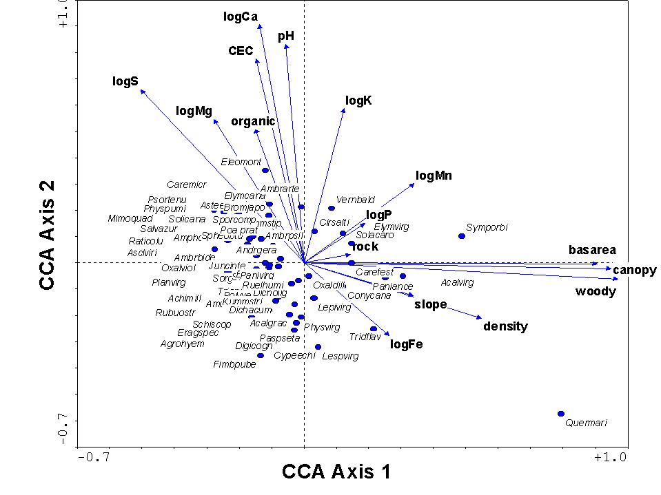
In general, we can conclude from the above that there are two
dominant factors (or at least, two factors related to variables we measured)
controlling vegetation at the Tallgrass Prairie Preserve: one is related
to forest vs. open conditions, and the other is related to soil acidity.
It seems that these two factors are relatively unrelated to each other,
since they are roughly orthogonal (at right angles) to each other.
In some cases, we might be interested in testing whether two different
groups of variables are redundant with each other, or whether they each
explain unique aspects of species composition. This is the purpose
of Partial Ordination. However, we can
go even further, and to partition the variance (i.e. inertia) into components:
-
A) That variance uniquely described by the first group (but not
explained by the second)
-
B) That variance uniquely described by the second group (but not
by the first)
-
C) That variance jointly described by both groups
-
D) That variance that is unexplained
Such a procedure is called variance partitioning or variation partitioning.
Although I briefly summarize the procedure here, please see the references
below for more details. Suppose we wish to calculate these variances
from the Tallgrass prairie data, and subdivide our data into "Soil" (variables
7-16) and "Other" (variables 1-6). Thus we can relabel A through
D above as:
-
A) S|O
-
B) O|S
-
C) OÇS
-
D) TI - OÈS
Where S and O refer to Soil and Other;
"|" means "given", or synonymously "factoring out" or "covarying out";
"Ç" refers to the intersection;
"TI" for the total inertia;
" È" for union.
In our case, we already have TI; it is 2.725. We also have OÈS,
since our CCA included both sets of variables. OÈS
is 0.776. Therefore, our unexplained variation is TI - OÈS
= 2.725-0.776 = 1.949.
We obtain S|O from a partial ordination where the soil variables
are our environmental variables, and the other variables are our covariables.
Our summary table appears like this:
**** Summary ****
Axes
1 2 3
4 Total inertia
Eigenvalues
: .132 .065 .051 .033
2.725
Species-environment correlations :
.877 .794 .815 .740
Cumulative percentage variance
of species data
: 5.7 8.5 10.6
12.1
of species-environment relation:
34.9 52.0 65.4 74.2
Sum of all unconstrained eigenvalues
2.328
Sum of all canonical
eigenvalues
.379
The only number that remains the same as in our previous table is the
total inertia. S|O is sum of all canonical eigenvalues, or 0.379.
Likewise, we obtain O|S from a partial ordination where the "other"
variables are our environmental variables, and the soil variables are our
covariables. We get the following summary table:
**** Summary ****
Axes
1 2 3
4 Total inertia
Eigenvalues
: .155 .023 .021 .015
2.725
Species-environment correlations :
.839 .659 .733 .525
Cumulative percentage variance
of species data
: 7.1 8.2 9.1
9.8
of species-environment relation:
65.6 75.5 84.4 90.7
Sum of all unconstrained eigenvalues
2.185
Sum of all canonical
eigenvalues
.237
Therefore, O|S = 0.237.
Now only one value is missing, i.e. OÇS, or the variation which is explained
by the intersection both data sets. Another way of saying this is
the variation that is explained by the redundant portion of both data sets.
We can calculate this using numbers we already have:
OÇS = OÈS
- O|S - S|O = 0.776 - 0.237 - 0.379 = 0.160
In other words, the intersection of the two sets is the variation explained
together, minus the variation uniquely explained by each data set.
Since the value of OÇS is smaller
than O|S and S|O, we can conclude that the two sets of variable are not
very redundant in explaining species composition, and each set of variables
are largely explaining unique aspects of, or 'gradients in', species composition.
This is not very surprising to us, since we noticed from the CCA diagram
that the two sets were largely orthogonal. However, in many real
world situations, we do not have such a neat 2-dimensional result, and
it is often not clear whether redundant sets of variables do indeed explain
unique variation.
We can report our variance partitioning in the form of percentages and
pie charts:

We can also use the above to summarize each set of variables separately,
e.g. Soil explains 14%+6% or 20% of the variation in the data set, while
the other variables explain 9%+6%=15% of the variation. However,
we need to exert some caution in saying that soil is "more important" than
the other variables, for three reasons: 1) it is clear that the first CCA
axis is predominantly related to woody cover, 2) there are more soil variables
than the others, so it might be an artifact of variable number, and 3)
there are some general concerns about variance partitioning, to be discussed
shortly.
Some problems with variance partitioning
Since the variance we are partitioning in CCA is not really a true variance,
but rather an inertia, we run into certain potential problems. Instead
of detailing them in a list, I demonstrate them by example. Suppose
we have a (ridiculously) smooth noiseless coenocline, of identical species
evenly placed along a noiseless gradient. Furthermore, let us suppose
we sample evenly along this gradient:
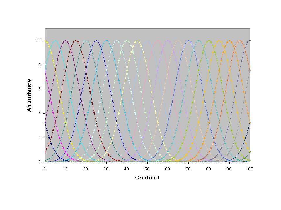
Let us also suppose that we have noiseless measures of the environmental
gradient. Of course, we never observe such a neat pattern in nature.
But if we did, this sort of gradient should be able to explain 100% of
the total inertia, or spread of species scores. But this is what
happens:
Axes
1 2 3
4 Total inertia
Eigenvalues
: .953 .842 .686 .514
3.927
Species-environment correlations :
.999 .000 .000 .000
Cumulative percentage variance
of species data
: 24.3 45.7 63.2 76.3
of species-environment relation:
100.0 .0 .0
.0
Sum of all unconstrained eigenvalues
3.927
Sum of all canonical
eigenvalues
.953
Since there is only one variable, then the first axis has 100% of the
cumulative variance of species-environment relation, but that would happen
even if the variable was random. The first eigenvalue is quite high,
which does suggest a very strong gradient. However, note that the
total variance explained, 0.953, is a small portion of the total inertia,
3.927. If we wished to calculate an equivalent of r2,
we would have 0.243. This is a pitifully small number, compared with
the 1.000 it should be!
One of the take-home messages of this is that an investigator should
not be disappointed if the variance explained seems small. It may
have nothing to do with nature.
What are the reasons for the low variance explained? I must admit
that it is hard to figure out completely (perhaps if we do, we will also
"solve" the arch effect), but here are some hints. Note that the
eigenvalue cannot exceed 1. This means that unless the total inertia
is less than 1, it is not possible to explain it all even with a perfect
eigenvalue. Also remember that Correspondence Analysis
suffers from the arch effect. Usually, CCA does not display an arch
because it is constrained by environmental variables which do not have
an arch-like structure. However, the tendency to form an arch is
still there, and can be seen in the unconstrained axes. In other
words, the arch itself can be said to have an inertia or variance.
In most real cases, we hope that this variance is part of the "unexplained"
variance, but it is indeed possible for at least part of it to show up
in the "explained" portion. Suppose we had a variable that did not
explain species composition, but happened to be correlated with a quadratic
function of the most important variable (i.e., it has an arch-like relationship
to the variable). Then this variable would erroneously appear as
important, AND cause an arch effect. In the example of the clean
gradient, when we include our variable and our variable squared, we get:
**** Summary ****
Axes
1 2 3
4 Total inertia
Eigenvalues
: .953 .818 .686 .533
3.927
Species-environment correlations :
.999 .993 .000 .000
Cumulative percentage variance
of species data
: 24.3 45.1 62.6 76.1
of species-environment relation:
53.8 100.0 .0 .0
Sum of all unconstrained eigenvalues
3.927
Sum of all canonical
eigenvalues
1.771
Note that the total variance explained jumps up substantially (from
0.953 to 1.771), even though the variable squared does not influence species
composition. In a sense, it is now "explaining" the arch.
The resulting CCA triplot appears as follows:
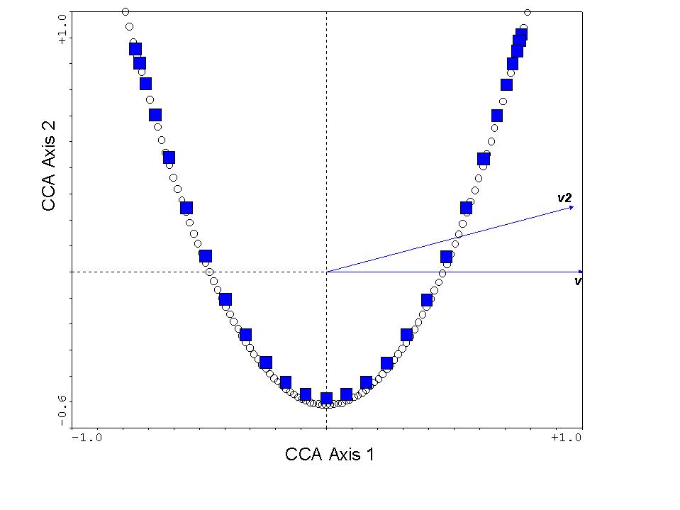
The squares are our species scores, the circles are the sample scores,
"v" is the variable representing the true gradient, and "v2" is this variable
squared. Not surprisingly, v is lying directly on the x-axis,
as it is the primary determinant of species composition. Also, v2
is highly correlated with v, so it points in roughly the same direction.
However, v2 is a nuisance variable, since it does not "explain" species
composition. Instead, it clearly "explains" the arch effect.
So the new, additional, variance explained is largely nonsensical.
Incidentally, v2 explains a highly "significant" amount additional
variance, after factoring out the effects of v (this testing is fairly
easy to do in CANOCO's manual forward selection). Also, v3
and v4 each explain "significant" additional variation.
Of course they all should not, since we have simulated the coenocline
in only one dimension. This teaches us to be cautious of:
-
Interpreting low "variance explained" as a poor fit of the model
-
Interpreting high "variance explained" as a good fit of the model
-
Including quadratic terms in a model
-
Interpreting "significance" of such terms
-
Inclusion of terms that have nonlinear relationships with important gradients
-
Interpreting "significance" of such terms
-
Variance partitioning in general
Rune Økland has independently discovered and analyzed some of the
problems listed above (Journal of Vegetation Science 10:131-136; 1999).
He proposes that in variance partitioning, we simply ignore the "unexplained
variance" term, and focus our decomposition of variance on only the "explainable"
variance, i.e. OÈS. I generally
agree with this advice, but still warn that the arch inertia may be lurking
somewhere in this "explainable" portion......
References on variance partitioning
Birks, H. J. B. 1996. Statistical approaches to interpreting diversity
patterns in the Norwegian mountain flora. Ecography 19:332-40.
Borcard, D., and P. Legendre. 1994. Environmental control and spatial
structure in ecological communities: an example using oribatid mites (Acari,
Oribatei). Environmental and Ecological Statistics 1:37-61.
Borcard, D., P. Legendre, and P. Drapeau. 1992. Partialling out the
spatial component of ecological variation. Ecology 73:1045-55.
Ohmann, J. L., and T. A. Spies. 1998. Regional gradient analysis and
spatial pattern of woody plant communities of Oregon forests. Ecol. Mon.
68:151-82.
Økland, R. H., and O. Eilertsen. 1994. Canonical correspondence
analysis with variation partitioning: some comments and an application.
J. Veg. Sci. 5:117-26.
Økland, T. 1996. Vegetation-environment relationships of boreal
spruce forests in ten monitoring reference areas in Norway. Sommerfeltia
22:349pp.
Wiser, S. K. 1998. Comparison of Southern Appalachian high-elevation
outcrop plant communities with their Northern Appalachian counterparts.
J. Biogeogr. 25:501-13.
This page was produced and is maintained by Michael Palmer.
 To
the ordination web page
To
the ordination web page