Statistics

The word "Statistics" is variously defined by statisticians - but is usually used in the context of testing null hypotheses.  Some use "statistics" to include ordination and classification.

---

Suppose we are interested in the effects of fertilization and lake area on the species richness of invertebrates in a lake.

Lake	Species Richness	Area	Fertilized
1	32	2.0	1
2	29	0.9	1
3	35	3.1	1
4	36	3.0	1
5	41	1.0	0
6	62	2.0	0
7	88	4.0	0
8	77	3.5	0
mean	50	2.4375	0.5
SD	22.6	1.1426	0.535

Is there an effect of fertilization on species richness? To answer this, we need to set up a Null Hypothesis:
H₀: m _f = m _nf
m (the Greek letter mu) is a symbol that represents the true mean of the population. We can never know it, but we can estimate it (using the simple average), and make inferences about it.

We calculate t according to the formula:

          _    _ 
         |x1 - x2| 
t = --------------------      = 3.302 
    [(s21/N1 + s22/N2)]0.5

      _
where x₁ is the mean of group 1 (pronounced "x-bar-sub-one"), s²₁ is the variance of group 1, and N₁ is the sample size of group 1.

Looking this number up in a t-table with N-2 = 6 degrees of freedom, we find that p<0.05. We reject H₀.
______________________________________________________

TESTING FOR CORRELATIONS BETWEEN VARIABLES

Correlation tests relationships between two variables. You need to identify an independent variable (x variable) which is often considered the causative agent, and a dependent variable (y variable) which is thought to be affected by x.

For example, x might equal the number of leaves on a dandelion plant produced in the fall, and y might equal the number of flower heads produced in the spring. We might expect more flowers to be produced if the plant had more leaves during the past growing season - this might be because plants with many leaves would have more carbohydrates stored up for reproduction.

Our null hypothesis is that the number of leaves is unrelated to the number of flowerheads. In other words,

H₀: x is uncorrelated with y
H₁: x is correlated with y
If a graph is made, the x variable is typically plotted on the x (horizontal) axis and the y variable is plotted on the y (vertical) axis. A simple equation (given later) results in a value known as r or the correlation coefficient. r takes values from -1 to +1.

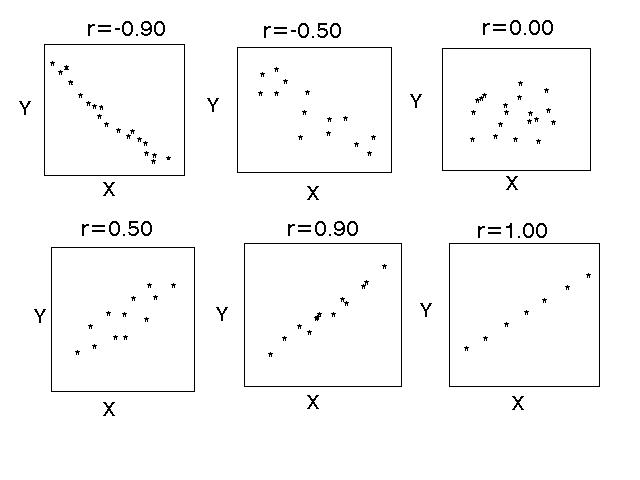
Note that values close to -1 and +1 indicate very strong relationships, those close to zero indicate very weak relationships. Negative r's indicate negative relationships; positive r's indicate positive relationships. A value of zero indicates no relationship between the variables. Another way of restating our null hypothesis is that the correlation coefficient will equal zero, and our alternative hypothesis is that the coefficient will differ significantly from zero.

r² has a special meaning: The proportion of variance in y which can be accounted for, or explained, by x.

The following is the formula for r:

              _     _
S(x_i-x)(y_i-y)
r = ________________________
            _        _
     {[S(x_i-x)²][S(y_i-y)²]}^0.5

Now that we have r, how do we know if it is significantly different from zero? We must first convert our r into a value of t using the following formula:
t = |r| [(N-2)/(1-r²)]^0.5
We now look up this value of t in the t table with N-2 degrees of freedom, in a way very similar to that done for the t-test.
One important thing to remember about correlation is that it does not necessarily imply direct causation.

---

USING REGRESSION TO FIT LINES TO DATA

As previously discussed, correlation is the process of finding the strength of the relationship between variables. Furthermore, correlation results in a measure of the significance (i.e. a statistical test) of the relationship. However, scientists often wish to move beyond simply testing, and would like to find a mathematical function which models the relationship. This modelling process is termed regression (more colloquially known as "line fitting" or "curve fitting").

This section describes linear least-squares regression, which fits a straight line to data. If a variable y is linearly related to x, then we use the formula for a line:

^
y = mx + b

Or more commonly in the context of regression,

^
y = b₀ + b₁x
where b₁ is the slope of the line, and b₀ is the y-intercept. Note that the y has a caret (^) over it. This is pronounced "y-hat" and means it is our estimated value of y. We need this symbol because is because it is extremely rare for actual data points to fall exactly on a line.

We can express this same equation differently as
y = b₀ + b₁x + e     for the function , or

y_i = b₀ + b₁x_i + e_i for a particular pair of x's and y's.  The term e_i is the residual for observation i; that is, the difference between the prediction and the observed value.  Note that the 'hat' is gone for the y.

We take b₀ and b₁ to be estimates of two abstract parameters in the equation:
y = ß₀ + ß₁x + e for the function, or
y_i = ß₀ + ß₁x_i + e _i for a particular value.
e is considered "error", and is not knowable.

The regression  function is not knowable, but we wish to make inferences about it. The larger our sample size, the more confident we are about our function, as long as the assumptions are correct.
The assumptions include:

• errors (e ) are independent of each other
• errors are normally distributed, and centered around the true value
• the underlying model is correct!

Once we know the mean and standard deviation for x and y, and the correlation coefficient (r) between them, we can calculate b₀ and b₁:
b₁ = r * s_y / s_x
     _     _
b₀ = y - b₁x

where x-bar and y-bar are the means of x and y, respectively, s_x and s_y are the standard deviations of x and y, respectively, and r is the correlation coefficient of the relationship between x and y.

Note that both b₁ and b₀ have units associated with them; they are not dimensionless.  The slope will be in units of y-units divided by x-units, and the intercept will be in y-units.  Also note that r must have the same sign as b_1.

In other words, if r is positive, the slope must be positive, and if r is negative, the slope must be negative.  NOTE: this is not to be confused with the capital R, the multiple correlation coefficient, which must always be positive.  Sometimes computer programs provide you only with R and not r.

By performing the appropriate calculations, the fitted regression function for the invertebrate example turns out to be:

^
y = 18.5 + 12.9x

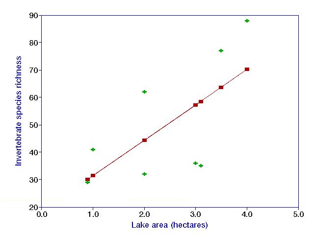
The above figure displays data (green crosses), as well as the fitted regression line (through the red squares, our "y-hats"). Note that the line fits the data fairly well. However, given that our sample is incomplete (we have not collected data from all possible lakes), the data have a little bit of randomness involved with them. We can therefore never say the line we find is the "real" or "true" line (This is akin to the reason we can never truly accept the null hypothesis).

However, we can say that the line is our best hypothesis of the relationship between x and y, given the assumption that the variables are linearly related. Often relationships are not linear; in this case more sophisticated techniques are needed.  We know in this particular case that the assumption is technically incorrect, since the model predicts 18.5 species when the lake area is zero, which appears to be a nonsensical result.  But in most cases, we are not too concerned with misbehavior of the model outside the range of our data.

How is the calculated line our "best" hypothesis?  The technique chooses the one line, out of all possible lines, which is closest to all the data points. In particular, the sum of the squares of the vertical distances between the line and the data points is as small a number as possible:
 N     ^
S (y_i-y_i)² is smallest, given the data.
i=1
The fact that the difference is squared is the reason the technique is called linear least-squares regression.

The quantity:

    ^
(y_i-y_i) has another name: the residual  (often abbreviated e_i).   The residual is taken as a measure of the abstract parameter e _i , or true error, mentioned previously.  Of course, 'error' is not to be interpreted to imply mistakes or sloppiness - though such is not be ruled out entirely, either.

---

Variables are often in different units, so how can they be compared?

They can be standardized:

Ranks - Data are sorted by value, and the values are replaced by the order in which the data points are listed. 1 = lowest value, N= highest value, and ties are given the tie of the ranks.

Logarithms

A constant unit equals a constant multiple on the arithmetic scale. For example, A tenfold difference in length will be the same distance apart as a tenfold difference in dollars. The difference between 1g and 30g will be the same distance as 1 ton and 30 tons. Logarithms are not defined for values of zero or less.  Therefore, sometimes people add a number (such as 1) before taking the logarithm.  However, this practice does not result in a true standardization.

Standardized to maximum

New value = value/maximum
This only makes sense when the minimum possible value is zero.

Standardized to 0-1 range:

New value = (value-min)/(max-min)
This transformation is used in Fuzzy Set Theory.

Standardized by subtracting the mean, then dividing by the standard deviation.

This is the most common way to standardize, and it has some nice mathematical properties. The mean equals zero, and the standard deviation AND the variance equals 1.
If you standardize all variables by this method, you don't have to worry about y-intercepts!
This is because:

   _   _
b₀=y-b₁x
b₀=0-b₁(0)=0

Note: the last three methods of standardization are linearly related to the raw data.

"Standardization" is a special case of "transformation", but is special in that it has no units, and therefore we can compare variables that were originally measured in different units.

---

This page was created and is maintained by Mike Palmer.
To the Ordination Web Page