Correspondence Analysis

Principal Components Analysis (PCA) suffers from a serious problem, the horseshoe effect, which makes it unsuitable for most ecological data sets. The problem is caused by the fact that species often have unimodal species response curves along environmental gradients. PCA assumes that species are linearly (or at least monotonically) related to each other, and to gradients.

The reason PCA fails is that it represents sample occurrences in species space (See Similarity, Difference and Distance). Correspondence Analysis (as well as its derivatives) represent species AND samples as occurring in a postulated environmental space, or ordination space. Correspondence Analysis (CA) assumes that species have unimodal species response curves. A species is located in that location of space where it is most abundant.

There are a number of different algorithms for CA (see Terminology in Ordination), but the most widely described is the Reciprocal Averaging algorithm (hence, CA is often called Reciprocal Averaging or RA). This algorithm proceeds as follows:

1. assign arbitrary numbers to all of your species. These numbers can be random numbers. These are your trial species scores.

2. create trial sample scores as follows: for each sample, calculate the weighted average of all of the species scores. The "weights" are x_ij, or the abundance of each species j in each sample i:

• sample score_i = S(x_ij * species score_j) / S(x_ij) Where the summations are over all species j

3. create new species scores as the weighted average of all the sample scores:

• species score_j = S(x_ij * sample score_i) / S(x_ij) Where the summations are over all samples i

4. restandardize species scores and sample scores by subtracting the mean and dividing by the standard deviation (though other kinds of standardization are possible here).

5. repeat steps 2-4 until there are almost no changes in successive iterations.

The above procedure results in first axis species scores and first axis sample scores, simultaneously ordinated along the SAME first axis. The second and higher axes can be calculated in a similar way, except extra steps are included to insure that these axes are uncorrelated (or orthogonal) to the first axis.

The above algorithm seems like circular reasoning: You start with meaningless numbers, then just average them in a fancy way, and expect to find a meaningful pattern! Well, it turns out that a meaningful pattern arrives because:

1. you will get the same results no matter what your starting point of species scores (i.e. you are guaranteed to find "convergence").
2. The end result is that Species scores and sample scores will be maximally correlated with each other (that is, we could not hope for a better solution, given the data).
3. The eigenvalue is a measure of how well the species scores correspond with the sample scores (hence the name Correspondence Analysis). In particular, the eigenvalue of an axis will equal the correlation coefficient between species scores and sample scores.
4. This first axis usually turns out to be related to important environmental gradients.

Let us repeat the example of the Boomer Lake study, in which species appear to be related to position above the lakeshore. For other examples of the use of this data set, see Explorations in Coenospace and Principal Components Analysis.

The first two axes of the correspondence analysis solution are shown below:

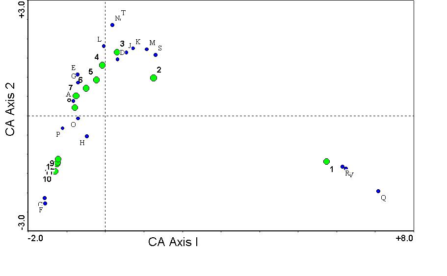
The first through the fourth eigenvalues are 0.7791, 0.5524, 0.3075, and 0.1628 respectively. These cannot be interpreted as "variance explained" as cleanly as in the case of PCA, but they can instead be explained as the correlation coefficient between species scores and sample scores, as indicated above and below.

There are several things to note with this diagram:

• Both species scores (blue circles, labeled with letters) and sample scores (green circles labeled with numbers) are graphed simultaneously. This is therefore called a biplot. (Note: only the most abundant species are plotted, although all species were used in the analysis).
• The centroid of sample scores and species scores is zero along all axes.
• Sample 1 (on the right) is distinctly different from sample 2, and all samples are arranged in sequential order from left to right (except for a slight jumble at the far left due to noise). Recall that sample 1 is actually in the lake, and sample 12 is far away.
• Species are located closely to the samples they occur in. If you looked carefully into the data matrix, you would find that species R and Q are strictly aquatic, while species F is a dryland plant.
• There is an arch effect. This is not as extreme as the horseshoe effect in PCA.
• Although it is difficult to tell here (contrast these results with the clearer examples in Gauch (1982) and Pielou (1984)), there is some compression of the gradient along the first axis. This is only evident on the left end here. If you only looked at the behavior of samples 4-12 only along the first axis (i.e. ignoring the second), they would be much closer together.

We mentioned that the correlation between species scores and sample scores is maximized. What do we mean by this? Well, let us first take a look at the raw data matrix: The rows are listed in alphabetical order of the species names (given short codes here for convenience, as in the figure above). The columns are listed in sequence of quadrats, from in the water (Q1) to up on dry land (Q12). Note that it is difficult to see a unified trend or structure in the data set.

SPECIES	Q!	Q2	Q3	Q4	Q5	Q6	Q7	Q8	Q9	Q10	Q11	Q12
A	0	0.99	4.52	19.8	27.49	23.74	21.16	15.4	2.95	6.36	20.16	16.65
B	0	0	0	0	3.01	7.3	8.53	11.76	23.13	25.61	22.09	32.01
C	0	0	0	0	0	0	0	5.59	22.26	23.17	30.06	25.67
D	0	23.15	19.16	5.54	3.91	1.52	0	5.74	3.47	1.76	2.26	1.81
E	0	0	1.75	5.23	6.72	17.34	19.32	6.88	3.36	0	0	0
F	0	0.99	0	0	0	0	0	0	18.43	19.48	14.06	3.9
G	0	2.12	5.66	1.48	0	0	14.57	18.39	2.72	0	0	0
H	2.41	3.94	0	0.8	2.33	3.05	6.45	5.89	3.47	5.29	4.52	5.44
I	33.95	7.75	0	0	0	0	0	0	0	0	0	0
J	2.41	7.22	6.18	5.94	6.72	9.53	1.61	0	0	0	0	0
K	2.41	8.36	6.15	7.41	8.5	4.96	0	0	0	0	0	0
L	0	5.39	10.85	5.92	0	2.34	5.95	6.26	0	0	0	0
M	2.74	11.48	6.57	4.57	8.09	1.52	0	0	0	0	0	0
N	0	3.11	13.9	10.02	4.38	3.32	0	0	0	0	0	0
O	0	2.73	1.65	2.54	6.16	3.05	0	0	0	5.39	4.6	3.63
P	0	0	0	0.8	1.17	5.51	5.07	1.66	1.68	3.62	0	5.44
Q	22.06	1.14	0	0	0	0	0	0	0	0	0	0
R	17.93	3.72	0.83	0	0	0	0	0	0	0	0	0
S	2.41	5.16	3.41	4.56	2.33	1.52	0	0	0	0	0	0
T	0	2.43	7.6	5.79	1.37	0	0	0	0	0	0	0
U	0	0	0	3.23	4.32	0	1.61	4.08	3.94	0	0	0
V	13.68	2.28	0.83	0	0	0	0	0	0	0	0	0
W	0	0	0	0	1.78	3.44	3.64	3.18	0	0	0	0
X	0	0.99	0.83	4.03	1.78	0	0	1.66	2.72	0	0	0
Y	0	0	0	1.61	0	0	0	1.66	3.36	0	2.26	1.81
Z	0	0.99	0	0	2.33	0	1.8	0	1.68	2.25	0	0
AA	0	0	0	0	0	3.98	0	3.13	0	1.76	0	0
BB	0	0	0	0	0	1.8	2.17	4.08	0	0	0	0
CC	0	0.99	2.48	1.21	1.78	1.52	0	0	0	0	0	0
DD	0	0.99	2.48	1.61	1.17	0	0	0	0	0	0	0
EE	0	0.99	0.83	2.41	0	0	0	0	0	0	0	1.81
FF	0	0.99	0	0	0	0	0	3.18	1.68	0	0	0
GG	0	0	1.75	2.15	0	0	0	0	1.68	0	0	0
HH	0	0	0	0.8	0	3.05	1.61	0	0	0	0	0
II	0	0	0	0	0	0	4.89	0	0	0	0	0
JJ	0	0	0	0	0	0	0	0	1.68	1.76	0	0
KK	0	0	0.83	0.8	0	0	1.61	0	0	0	0	0
LL	0	0	0	0	0	0	0	1.47	0	1.76	0	0
MM	0	0	0	0	1.17	1.52	0	0	0	0	0	0
NN	0	0	0	0	0	0	0	0	0	0	0	1.81
OO	0	0	0	0	0	0	0	0	1.79	0	0	0
PP	0	0	0.83	0.94	0	0	0	0	0	0	0	0
QQ	0	0	0	0	0	0	0	0	0	1.76	0	0
RR	0	0	0	0	1.17	0	0	0	0	0	0	0
SS	0	0	0	0	1.17	0	0	0	0	0	0	0
TT	0	0	0	0	1.17	0	0	0	0	0	0	0
UU	0	1.14	0	0	0	0	0	0	0	0	0	0
VV	0	0.99	0	0	0	0	0	0	0	0	0	0
WW	0	0	0.93	0	0	0	0	0	0	0	0	0
XX	0	0	0	0.8	0	0	0	0	0	0	0	0

Now let us arrange our columns in order of ascending sample score, and our rows in order of ascending species score. The first row consists of the sample scores.

		-1.2979	-1.245	-1.2282	-1.216	-0.7842	-0.7549	-0.4922	-0.225	-0.0658	0.3083	1.2607	5.7394
Species	Species score	Q10	Q11	Q9	Q12	Q8	Q7	Q6	Q5	Q4	Q3	Q2	Q1
QQ	-1.6658	1.76	0	0	0	0	0	0	0	0	0	0	0
JJ	-1.6222	1.76	0	1.68	0	0	0	0	0	0	0	0	0
OO	-1.5765	0	0	1.79	0	0	0	0	0	0	0	0	0
C	-1.5683	23.17	30.06	22.26	25.67	5.59	0	0	0	0	0	0	0
NN	-1.5608	0	0	0	1.81	0	0	0	0	0	0	0	0
F	-1.5557	19.48	14.06	18.43	3.9	0	0	0	0	0	0	0.99	0
B	-1.4236	25.61	22.09	23.13	32.01	11.76	8.53	7.3	3.01	0	0	0	0
LL	-1.3657	1.76	0	0	0	1.47	0	0	0	0	0	0	0
Y	-1.2654	0	2.26	3.36	1.81	1.66	0	0	0	1.61	0	0	0
P	-1.1078	3.62	0	1.68	5.44	1.66	5.07	5.51	1.17	0.8	0	0	0
AA	-0.9692	1.76	0	0	0	3.13	0	3.98	0	0	0	0	0
II	-0.9689	0	0	0	0	0	4.89	0	0	0	0	0	0
BB	-0.9126	0	0	0	0	4.08	2.17	1.8	0	0	0	0	0
A	-0.8207	6.36	20.16	2.95	16.65	15.4	21.16	23.74	27.49	19.8	4.52	0.99	0
Z	-0.7968	2.25	0	1.68	0	0	1.8	0	2.33	0	0	0.99	0
W	-0.782	0	0	0	0	3.18	3.64	3.44	1.78	0	0	0	0
U	-0.7798	0	0	3.94	0	4.08	1.61	0	4.32	3.23	0	0	0
FF	-0.726	0	0	1.68	0	3.18	0	0	0	0	0	0.99	0
E	-0.7192	0	0	3.36	0	6.88	19.32	17.34	6.72	5.23	1.75	0	0
O	-0.7007	5.39	4.6	0	3.63	0	0	3.05	6.16	2.54	1.65	2.73	0
G	-0.698	0	0	2.72	0	18.39	14.57	0	0	1.48	5.66	2.12	0
HH	-0.651	0	0	0	0	0	1.61	3.05	0	0.8	0	0	0
MM	-0.4826	0	0	0	0	0	0	1.52	1.17	0	0	0	0
H	-0.4752	5.29	4.52	3.47	5.44	5.89	6.45	3.05	2.33	0.8	0	3.94	2.41
X	-0.4066	0	0	2.72	0	1.66	0	0	1.78	4.03	0.83	0.99	0
KK	-0.401	0	0	0	0	0	1.61	0	0	0.8	0.83	0	0
GG	-0.3831	0	0	1.68	0	0	0	0	0	2.15	1.75	0	0
RR	-0.2887	0	0	0	0	0	0	0	1.17	0	0	0	0
SS	-0.2887	0	0	0	0	0	0	0	1.17	0	0	0	0
TT	-0.2887	0	0	0	0	0	0	0	1.17	0	0	0	0
EE	-0.1818	0	0	0	1.81	0	0	0	0	2.41	0.83	0.99	0
XX	-0.0845	0	0	0	0	0	0	0	0	0.8	0	0	0
L	-0.0281	0	0	0	0	6.26	5.95	2.34	0	5.92	10.85	5.39	0
CC	0.1262	0	0	0	0	0	0	1.52	1.78	1.21	2.48	0.99	0
PP	0.1407	0	0	0	0	0	0	0	0	0.94	0.83	0	0
N	0.1821	0	0	0	0	0	0	3.32	4.38	10.02	13.9	3.11	0
D	0.3201	1.76	2.26	3.47	1.81	5.74	0	1.52	3.91	5.54	19.16	23.15	0
DD	0.3375	0	0	0	0	0	0	0	1.17	1.61	2.48	0.99	0
T	0.3522	0	0	0	0	0	0	0	1.37	5.79	7.6	2.43	0
WW	0.3956	0	0	0	0	0	0	0	0	0	0.93	0	0
J	0.5518	0	0	0	0	0	1.61	9.53	6.72	5.94	6.18	7.22	2.41
K	0.7277	0	0	0	0	0	0	4.96	8.5	7.41	6.15	8.36	2.41
M	1.0774	0	0	0	0	0	0	1.52	8.09	4.57	6.57	11.48	2.74
S	1.3117	0	0	0	0	0	0	1.52	2.33	4.56	3.41	5.16	2.41
UU	1.6181	0	0	0	0	0	0	0	0	0	0	1.14	0
VV	1.6181	0	0	0	0	0	0	0	0	0	0	0.99	0
R	6.1579	0	0	0	0	0	0	0	0	0	0.83	3.72	17.93
V	6.2414	0	0	0	0	0	0	0	0	0	0.83	2.28	13.68
I	6.2982	0	0	0	0	0	0	0	0	0	0	7.75	33.95
Q	7.0841	0	0	0	0	0	0	0	0	0	0	1.14	22.06

Now the data matrix has a definite data structure. Species with low first axis scores (dryland species) tend to occur in samples with low first axis scores (dryland quadrats), and vice versa. Species with intermediate tolerances are closer to the centroid (i.e. scores close to zero), and samples with intermediate conditions also have scores close to the centroid. Numbers tend to be clustered around the diagonal. Thus there is a correspondence between species and samples in the above data.

Compare the above example with Gauch (1982) figures 4.9 and 4.10 and Pielou (1984) Table 4.11.

Now we will plot first axis species scores as a function of first axis sample scores:

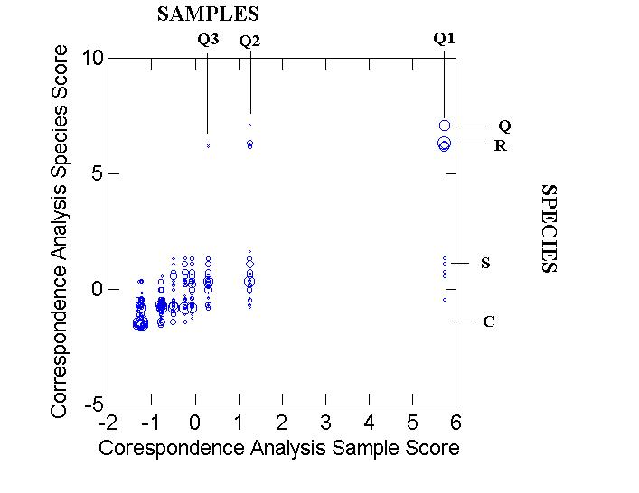
Here, the abundance of the species is proportional to the size of the circle, and zero abundances (i.e. absences) are not plotted. Note that there is a correlation between species scores and sample scores. In fact, the correlation is the MAXIMUM POSSIBLE correlation, given the data. The weighted correlation coefficient of the above scatter diagram will be equal to the eigenvalue of the first axis, which is 0.7791. A few samples (columns) and species (rows) are pointed out, note their relationships to the above data matrices. For example, Q and R are both wetland species (high first axis scores) which occur in the wettest quadrats, Q1 and Q2.

---

This page was created and is maintained by Michael Palmer.
To the ordination web page