MULTIPLE
REGRESSION
(Note:
CCA is a special kind of multiple regression)
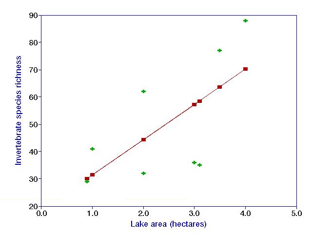
The
below represents a simple, bivariate linear regression on a hypothetical data
set.
The green crosses are the actual data, and the red squares are the
"predicted values" or "y-hats", as estimated by the
regression line. In least-squares regression, the sums
of the squared (vertical) distances between the data points and the
corresponding predicted values is minimized.
However, we are often interested in testing whether a dependent variable (y)
is related to more than one independent variable (e.g. x1,
x2, x3).
We could perform regressions based on the following models:
y = ß0 + ß1x1 + e
y = ß0 + ß2x2 + e
y = ß0 + ß3x3 + e
And indeed, this is commonly done. However it is
possible that the independent variables could obscure each other's effects. For
example, an animal's mass could be a function of both age and diet. The age
effect might override the diet effect, leading to a regression for diet which
would not appear very interesting.
One possible solution is to perform a regression with one independent variable, and then test whether a second independent variable is related to the residuals from this regression. You continue with a third variable, etc. A problem with this is that you are putting some variables in privileged positions.
A multiple regression allows the simultaneous testing and modeling of multiple independent variables. (Note: multiple regression is still not considered a "multivariate" test because there is only one dependent variable).
The model for a multiple regression takes the form:
y = ß0 + ß1x1 +
ß2x2 + ß3x3
+ ..... + e
And we wish to estimate the ß0, ß1, ß2,
etc. by obtaining
^
y1
= b0 + b1x1 + b2x2
+ b3x3 + .....
The b's are termed the "regression coefficients". Instead of fitting a line to data, we are now fitting a plane (for 2 independent variables), a space (for 3 independent variables), etc.
The estimation can still be done according the principles of linear least
squares.
The formulae for the solution (i.e. finding all the b's)
are UGLY. However, the matrix solution is elegant:
The model is: Y = Xß
+ e
The solution is: b =(X'X)-1X'Y
(See
for example, Draper and Smith 1981)
As with simple regression, the y-intercept disappears if all variables are standardized (see Statistics) .
LINEAR COMBINATIONS
Consider the model:
y = ß0 + ß1x1 +
ß2x2 + ß3x3
+ ..... + e
Since y is a combination of linear functions, it is termed a linear
combination of the x's. The
following models are not linear combinations of the x's:
y = ß0 + ß1/x1 + ß2x22
+ e
y = exp(ß0 + ß1x1
+ ß2x2 + ß3x3
+ e)
But you can still use multiple regression if you
transform variables. For the first example, create two new variables:
x1' = 1/x1 and x2' = x22
For the second example, take the logarithm of both sides:
log(y) = ß0 + ß1x1+
ß2x2 + ß3x3
+ e
There are some models which cannot be "linearizable",
and hence linear regression cannot be used, e.g.:
y = (ß0 - ß1x1)/3x2
+ e
Or, subtly,
y = exp(ß0 + ß1x1
+ ß2x2 + ß3x3)
+ e
These must be solved with nonlinear regression techniques. Unfortunately, it is hard to find the solution to such nonlinear equations if there are many parameters.
What
about polynomials?
Note that:
y = ax3 + bx2 + cx + d + e
can be expressed as:
y = ß0 + ß1x1+ ß2x2
+ ß3x3 + e
if x1 = x1, x2 = x2, x3 = x3
So polynomial regression is considered a special case of
linear regression. This is handy, because even if polynomials do not
represent the true model, they take a variety of forms, and may be close
enough for a variety of purposes.
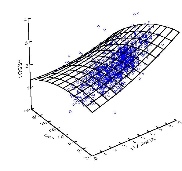
If you have two variables, it is possible to use polynomial terms and
interaction terms to fit a response surface:
y = ß0 + ß1x1+ ß2x12
+ ß3x2 + ß4x22
+ ß4x1x2 + e
This function can fit simple ridges, peaks, valleys, pits, slopes, and saddles. We could add cubic or higher terms if we wish to fit a more complicated surface.
ß4x1x2 is considered an interaction term, since variables 1 and variable 2 interact with each other. If b4 ends up being significantly different from zero, then we can reject the null hypothesis that there is 'no interaction effect'.
Statistical
inference
Along with a multiple regression comes an overall test
of significance, and a "multiple R2" - which is
actually the value of r2 for the measured y's vs. the
predicted y's. Most packages provide an
"Adjusted multiple R2" which will be discussed
later.
For each variable, the following is usually provided:
- a regression coefficient (b)
- a standardized regression coefficient (b if all
variables are standardized)
- a t value
- a p value
associated with that t value.
The
standardized coefficient is handy: it equals the value of r between the
variable of interest and the residuals from the regression, if the variable
were omitted.
The significance tests are conditional: This means given all the other variables are in the model. The null hypothesis is: "This independent variable does not explain any of the variation in y, beyond the variation explained by the other variables". Therefore, an independent variable which is quite redundant with other independent variables is not likely to be significant.
Sometimes, an ANOVA table is included.
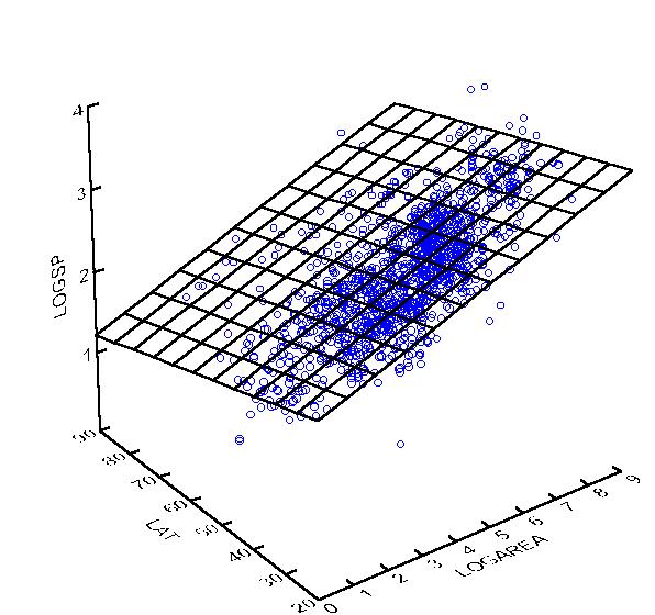
The following is an example SYSTAT output of a multiple regression:
Dep Var: LOGSP N: 1412 Multiple R: 0.7565 Squared multiple R: 0.5723
Adjusted squared multiple R: 0.5717 Standard error of estimate: 0.2794
Effect Coefficient Std Error Std Coef Tolerance t P(2 Tail)
CONSTANT 2.4442 0.0345 0.0 . 70.8829 0.0000LOGAREA 0.1691 0.0040 0.7652 0.9496 42.7987 0.0000LAT -0.0136 0.0008 -0.2993 0.9496 -16.7381 0.0000
Analysis of Variance
Source Sum-of-Squares DF Mean-Square F-Ratio PRegression 147.1326 2 73.5663 942.6110 0.0000
Residual 109.9657 1409 0.0780
It is possible for some variables to be significant with simple regression, but
not with multiple regression. For example:
Plant species richness is often correlated with soil pH, and it is often strongly correlated with soil calcium. But since soil pH and soil calcium are strongly related to each other, neither explains significantly more variation than the other.
This is called the problem of multicollinearity (though whether it is a 'problem', or something that yields new insight, is a matter of perspective).
It is also possible that nonsignificant patterns in simple regression become significant in multiple regression, e.g. the effect of age and diet on animal size.
Problems
with multiple regression
Overfitting:
The
more variables you have, the higher the amount of variance you can explain.
Even if each variable doesn't explain much, adding a large number of variables
can result in very high values of R2. This is why some
packages provide "Adjusted R2," which allows you to
compare regressions with different numbers of variables.
The same holds true for polynomial regression. If you have N data
points, then you can fit the points exactly with a polynomial of degree N-1.
The degrees of freedom in a multiple regression equals
N-k-1, where k is the number of variables. The more variables you
add, the more you erode your ability to test the model (e.g. your statistical power
goes down).
Multiple
comparisons:
Another
problem is that of multiple comparisons. The more tests you make, the higher
the likelihood of falsely rejecting the null hypothesis.
Suppose you set a cutoff of p=0.05. If H0 is
always true, then you would reject it 5% of the time. But if you
had two independent tests, you would falsely reject at least one H0
1-(1-.05)2 = 0.0975, or almost 10% of the time.
If you had 20 independent tests, you would falsely reject at least one H0
1-(1-.05)20 = 0.6415, or almost 2/3 of the time.
There are ways to adjust for the problem of multiple comparison, the most
famous being the Bonferroni test and the Scheffe test. But the Bonferroni
test is very conservative, and the Scheffe test is
often difficult to implement.
For the Bonferroni test, you simply multiply each
observed p-value by the number of tests you perform.
Holm's method for correcting for multiple comparisons is less well-known, and is also less conservative (see Legendre and Legendre, p. 18).
Partial
Correlation
Sometimes you have one or more independent variables which are not of interest,
but you have to account for them when doing further analyses. Such variables
are called "covariables", and an analysis which factors out their
effects is called a "partial analysis". Examples include:
- Analysis of Covariance
- Partial Correlation
- Partial Regression
- Partial DCA
- Partial CCA
(For
the simplest case, a partial correlation between two variables, A and B, with
one covariable C, is a correlation between the residuals of the regression of A on C and B on C. The only difference is in accounting for
degrees of freedom).
Examples: Suppose you perform an experiment in which tadpoles are raised at different temperatures, and you wish to study adult frog size. You might want to "factor out" the effects of tadpole mass.
In the invertebrate species richness example, Species Richness is related to area, but everyone knows that. If we are interested in fertilization effects, it might be justifiable to "cancel out" the effects of lake area.
Stepwise
Regression
Often, you don't really care about statistical inference, but would really like a regression model that fits the data well. However, a model such as:
y = ß0 + ß1x1 + ß2x2 + ß3x3 + ß4x4 + ß5x5 + ß6x6 + ß7x7 + ß8x8 + ß9x9 + ß10x10 + ß11x11 + ß12x12 + ß13x13 + ß14x14 + ß14x14 + e
Is far too ungainly to use! It might be much more useful to choose a subset of the independent variables which "best" explains the dependent variable.
There are three basic approaches:
1) Forward Selection
Start by choosing the independent variable which explains
the most variation in the dependent variable.
Choose a second variable which explains the most residual variation, and then
recalculate regression coefficients.
Continue until no variables "significantly" explain residual
variation.
2)
Backward Selection
Start with all the variables in the model, and drop the
least "significant", one at a time, until you are left with only
"significant" variables.
3)
Mixture of the two
Perform a forward selection, but drop variables which become
no longer "significant" after introduction of new variables.
In
all of th above, why is
"significant" in quotes? Because you are performing so many different
comparisons, that the p-values are compromised. In effect, at each
step of the procedure, you are comparing many different variables. But
the situation is actually even worse than this: you are selecting one model out
of all conceivable sequences of variables.
Although stepwise methods can find meaningful patterns in data, it is also notorious for finding false patterns. If you doubt this, then try running a stepwise procedure using only random numbers. If you include enough variables, you will almost invariably find 'significant' results.
This
page was created and is maintained by Michael
Palmer.
 To the ordination
web page
To the ordination
web page