Sampling and Experimental Design in Community Ecology

To consult the statistician after an experiment is finished is often merely to ask him to conduct a post mortem examination. He can perhaps say what the experiment died of. –Ronald Fisher

Designing an experiment properly will not only help you in analyzing data – it may determine whether you can analyze data at all!

The topic of experimental design is difficult to address – since community ecologists study such a wide range of systems and with unique qualities. Thus, sampling is largely idiosyncratic with respect to the community and organisms being studied. In addition, the optimal study design will largely depend on:

· The question(s) being addressed.

· Whether it is desirable to compare results to that of previous research

· Availability of suitable habitat or study sites

· Availability of suitable resources (time, money, equipment, helpers).

The first point above is the most important component of experimental design. However, it is also one of the most difficult ones for which to provide general advice – since novel questions will typically require novel sampling designs.

Nevertheless, there are some general principles I will quickly describe below.

Sampling in the field

While much of ecology has moved towards manipulative experiments, community ecology still depends upon observational experiments (note that some scientists incorrectly use the word ‘experiment’ to refer only to manipulative experiments. In reality, an experiment is a series of observations intentionally planned to address a scientific question).

One common criticism of observational experiments is that ‘correlation does not imply causation’. I disagree with this. Correlation implies causation. The problem is that we cannot infer the direction of causation without some scientific sleuthing. A correlation between soil organic matter and tree cover could be due to trees preferring organic soils, or leaf litter contributing to organic matter in the soil, or another variable simultaneously affecting tree distributions and organic matter.

It should be noted that causality is improperly inferred from many manipulative studies. A classic example (I hope it is fictional) is the scientist who trained frogs to jump on voice command, and incorrectly concluded that frogs are unable to hear when you remove their legs.

A key advantage of observational experiments is that they address how nature actually is, not what factors can be important.

In community ecology, the discipline of gradient analysis specifically addresses how species respond to spatial variation in the natural environment. Because of this, we need to pay special attention to how to place the samples in a spatial context.

With some exceptions below I will call an individual sample a ‘plot’, but note that many other types of samples are possible. I will also assume we are sampling on a 2-dimensional landscape, but note some exceptions, each with their own set of sampling issues:

· For some aquatic or soil organisms, we might more likely be sampling in 3 dimensions.

· For organisms associated with streams, coasts, or other more or less linear features, we are sampling along 1 dimension.

· Organisms dependent on other organisms (e.g. mosses on trees, phyllosphere bacteria) will require some form of point sampling

Despite all of these unique considerations, most of the principles below are still relevant.

Location of Plots

Subjective locations

If we are interested in observing species response to gradients, we might find it useful to insert our own natural history knowledge or intuition into plot locations. For example, if we wish to understand how species respond to gradients, it would be valuable to have the gradient extremes (e.g. very wet and very dry, or very steep and very level, or very acidic to very basic) if we wish to fully describe the responses of individual species. We may also want to have good representation of the intermediates. Having good representation of the gradients is not guaranteed with objective sampling. Subjective locations are also far easier to implement than objectively-located samples.

Typically plots are located to ensure within-plot homogeneity. This presumes the investigator’s intuition appropriately assesses homogeneity. There is a risk of ‘reification’ – that is, believing a community type is a real entity, sampling in such a way to maximize the distinctness and homogeneity of that community type, and then analyzing the data to highlight and demonstrate the existence of that community type. This is one of the main drawbacks of phytosociology.

Nevertheless, some kinds of heterogeneity can make inferred gradients messy and effectively decrease measured beta diversity (see Palmer, M. W. and P. M. Dixon. 1990. Small scale environmental variability and the analysis of species distributions along gradients. Journal of Vegetation Science 1:57-65.) An extreme case would be if a plot straddled the border between an oldfield and an old-growth forest, the ability to recover a successional pattern would be diminished.

Another drawback to subjective locations is that inferential statistics are invalid (though they tend nevertheless to be used in the literature). Also, the infusion of the investigator’s intuition into locating the plots makes the research non-replicable.

Gradsect

Often (but by no means always) we are interested in species responses to an environmental gradient that varies directionally in space. For example, we might be interested in bird species distributions as a function of elevation on a mountain, invertebrate species as a function of distance from a roadside, or mammal communities as a function of latitude. In such studies, we subjectively choose the gradient we are interested in a priori. It is often most productive then to locate our samples in a transect, systematically in a direction of maximum change in the gradient. Such transects are known as gradsects.

Below, I illustrate two kinds of gradsects along an elevational gradient. The blue squares represent contiguous quadrats in what we call a belt transect. They would perhaps be suitable for plant communities. The red dots represent point samples such as pitfall traps, and optimally would be placed at regular elevational intervals.

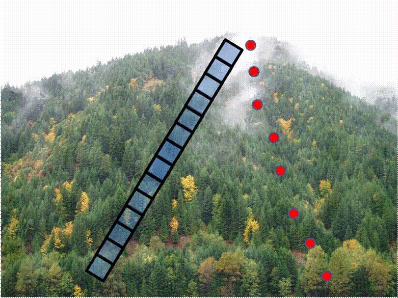
Note that there is a fair bit of faith involved in the gradsect approach: It is that any patterns we find are due to the gradient in question, rather than spatial dependence (discussed later). Since the gradient is linear and (in most cases) unreplicated, we will not be able to disentangle the pure effects of space from the effects of the gradient.

Also note that questions such as “Is there an elevational effect on species composition?” becomes uninteresting because you are presupposing it, and “Is elevation the most important environmental gradient in this landscape?” because the design strongly biases your answer.

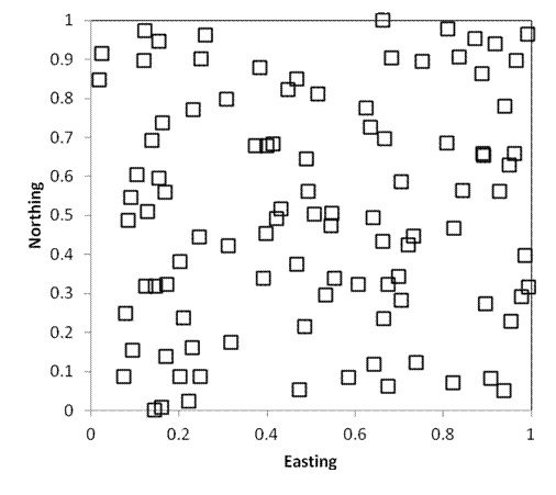
Completely random

Random plot locations circumvent problems of subjectivity (once once defines the sampling universe, which is a subjective decision). Ideally, every point in the sampling universe has an equal chance of being chosen.

Some investigators locate plots by throwing a rock over your shoulder, or walking a certain number of steps with their eyes closed. Not only are such techniques dangerous, they also do not represent random sampling. We call such techniques ‘haphazard’.

Instead, we use a random number generator on a computer or calculator. Technically these are pseudorandom because they use a deterministic algorithm, but they behave ‘as if random’. In Excel, we can generate a random number using the formula “=RAND()”, which chooses any number between 0 and 1 with equal likelihood. If we wish to find a random point in a rectangle 100m by 50m, we can use the formulae “=100*RAND()” and “=50*RAND()” to find x and y coordinates. It is fairly simple to generate random coordinates in R or using GIS Software. The map below illustrates random sampling of 100 plots in a hypothetical square 1km on each side.

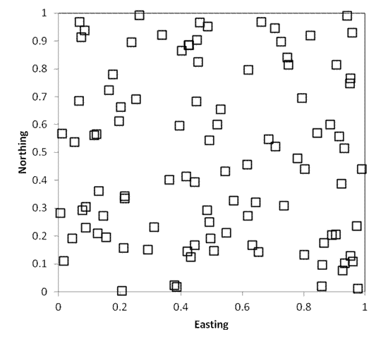
Sometimes, investigators wish to choose a random point within a circle. The commonly used technique of choosing a random direction and a random distance from the center will NOT result in a uniform probability of selecting any point in the circle, as points near the center will be more likely:

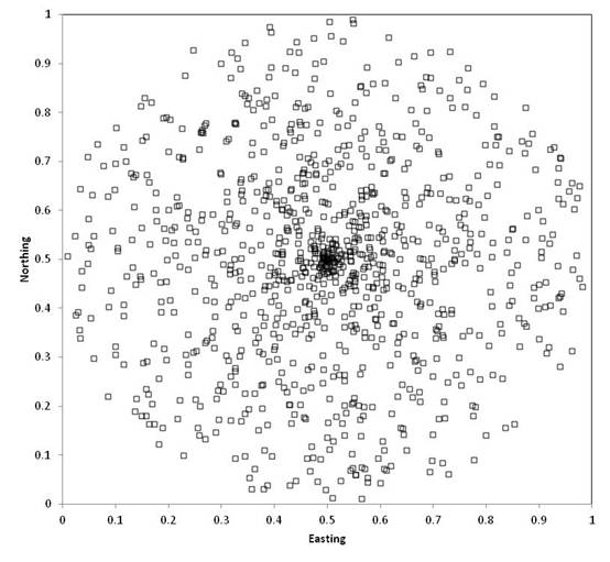
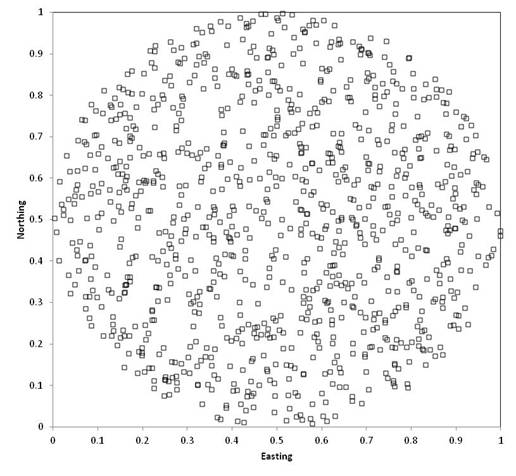
For a uniform distribution within a circle, you need to multiply the maximum radius by the square root of a uniform random number:

Generating random coordinates in irregularly-shaped universes is more difficult in most cases, though GIS routines exist. The simplest way to implement this is to use rectangular coordinates but reject points falling outside the sampled area.

Note that just due to chance, some areas will be oversampled and some areas will be undersampled. Stratified random sampling circumvents this.

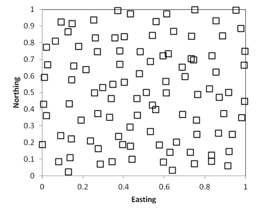
Stratified random

There are quite a few ways to conduct stratified sampling, but the two main ways are purely by space, or to also include landscape heterogeneity as a criterion.

Purely spatially

As in the preceding example, the following two sampling designs also include 100 samples randomly located within a square kilometer. Every point still has an equal chance of being sampled. However, in the first example below, 25 plots are randomly located in each quadrant (i.e. each quarter of the square). In the second example, 1 quadrat is located within each 100m x 100m grid cell of the study area. As you can see, stratified random sampling results in a more dispersed sampling, and decreases the likelihood that large areas will be randomly missed.

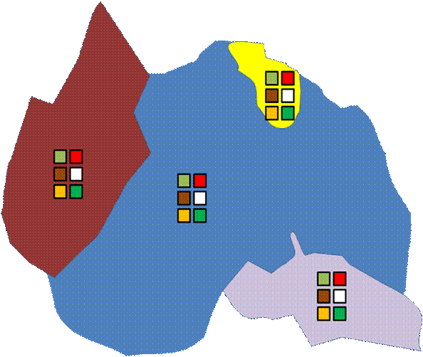
By landscape heterogeneity

Often, investigators wish to guarantee that all major elements of the landscape are included. In the below example, 5 plots are randomly located within each of five landscape units.

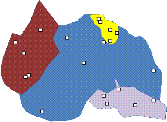
This does guarantee sampling of different habitat types (if the landscape is stratified by habitat). But note that we have forfeited our claim of objectivity. We have already stratified the landscape by what we consider important. Also, the boundaries on a map (especially if they are considered soil types or habitat delineations) are already the result of a number of subjective decisions.

Unlike spatial stratification, every point is not equally likely to be chosen. It is possible to rectify this by having the number of samples proportional to the area of habitat types. Nevertheless, the a priori classification of the sampling universe will strongly influence the results.

Systematic placement

If we are interested in analyzing or quantifying spatial pattern, it is often very useful to have a systematic design such as plots regularly spaced along a transect or rectangular grid (hexagonal arrays are also occasionally used). The plot locations are objective.

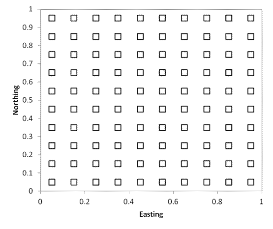
An additional advantage of this approach is that special techniques exist for analyses in rectangular grids.

A theoretical disadvantage of systematic placement is that it is possible that periodicity exists in nature, and that the spacing of plots coincides with this periodicity. However, this kind of spatial pattern is exceptionally rare in nature compared to ordinary distance decay (discussed later). It is easier to correct for such distance decay using a regular grid.

Randomly selecting entities

Often our sample consists of some sort of entity like an isolated habitat (e.g. island or rock outcrop) or an individual (e.g. a tree upon which we wish to study epiphytes, a plant from which we are isolating bacteria, etc.). Unless we sample the entire universe (e.g. all trees, all islands, all outcrops in the area) we need to objectively subsample.

One common way of subsampling is to randomly select a point, and then choose the closest individual to that point. While this seems logical and objective, it is biased: isolated individuals, or individuals on the outside edges of clumps, are far more likely to be selected than are individuals in the middle of clumps.

A better technique is to start by identifying all the individuals in the universe, to completely enumerate them, and then to randomly select individuals from the list. In cases where this is infeasible, one can select random individuals from a complete enumeration within objectively located plots.

Exclusion criteria

Objectively located plots can be problematic. For example, they can end up in locations that are either inconvenient or impossible to sample. Alternatively, they can end up in locations that may not be of interest (e.g. in the middle of a road). Or perhaps you are studying forests in a region with scattered glades that are not part of the study. Therefore, it is important to set up a priori criteria for excluding plots. In essence, you are defining your sampling universe as a subset of the entire area. But if you exclude areas from consideration a posteriori then you run the risk of introducing elements of subjectivity in your analysis.

Ecologists differ as to whether to reject plots that overlap in space. I believe they should be excluded before heading to the field, or better yet the algorithm to initially select plots can be adjusted to forbid overlap.

Practically speaking, one should bring extra random coordinates into the field for replacement plots, in case some are rejected.

Excluding plots in systematic grids or transects will limit the ability to use some kinds of spatial analyses.

Spatial dependence and Pseudoreplication

Random or systematic placement of plots does not guarantee that your plots are independent of each other. Indeed, according to Tobler’s first law of geography, nearby locations are on average more similar to each other than distant locations. In the context of spatial ecology, we call this spatial autocorrelation or spatial dependence.

Spatial dependence arises from a number of ordinary phenomena. For example, nearby areas may be chemically similar because they share the same bedrock. Simple geological processes will cause one point in a valley to have a similar elevation to a nearby point in the valley. Limited dispersal or clonal growth will cause plant or animal distributions to be spatially aggregated.

Let us imagine a field with spatially autocorrelated soil moisture, in this case being dry towards the left and moist towards the right. Let us also imagine that two ant colonies are founded at random locations. Any sort of localized sampling will tend to capture more ants in nearby colonies, resulting in spatially autocorrelated spacies composition.

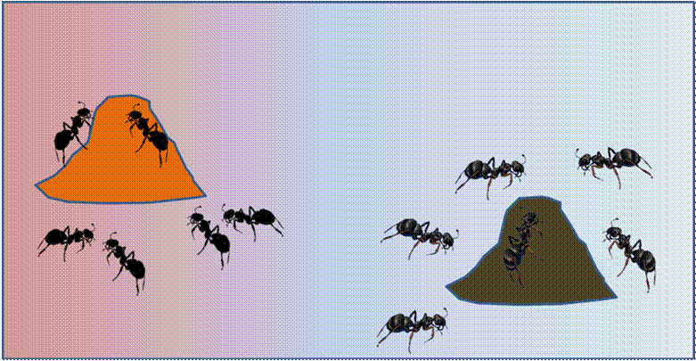
Even though the ants colonized the field randomly (that is, independent of the moisture gradient), we are virtually guaranteed to find a (false) relationship between soil moisture and species composition.

It is possible that a detailed study of the environment will allow one to find appropriate spatial scales at which to sample to avoid spatial dependence (Palmer, M. W. 1988. Fractal Geometry: a tool for describing spatial patterns of plant communities. Vegetatio 75:91-102.). However, in general the situation is difficult to avoid. The use of regular grids minimizes the problem (since samples have maximum dispersion) but even better, grids permit spatial permutations that can help correct for spatial dependence.

Most ecologists are aware of the important issue of pseudoreplication (Hurlbert, S. H. 1984. Pseudoreplication and the design of ecological field experiments. Ecological Monographs 54:187-211.). For example, having 100 samples in a burned area and 100 samples in an unburned area does not allow a valid test of fire effects, as the areas likely vary dramatically. In cases where pseudoreplication is unavoidable (e.g. if there is only one fire in the area) one can decrease its effects by (for example) having multiple transects (or paired plots) across the border between the areas, but the effects are still present and any sort of inferential statistics are highly suspect.

Most kinds of pseudoreplication can be considered an extreme form of spatial dependence.

Data quantity vs. quality

One of the first choices an investigator faces when designing a study is to decide how much data to collect associated with each plot, and how many plots to sample. There is an inevitable tradeoff, with respect to time and expense. It is my general observation that beginners sometimes underestimate the importance of replication, and spend a lot of time recording variables (some of which are unlikely to be important) in excruciating detail. It may be useful to devise quick proxies for variables that are difficult to measure. Often, high precision is unnecessary because among-site variation is orders of magnitude greater than measurement error.

Note also that sample size influences the number of questions you can expect to address. A sample size of 20 may be perfectly reasonable for testing the effects of soil pH on species composition. However, it will be completely inadequate if you wish to test the independent effects of 15 soil variables. For every variable that you add, you decrease your degrees of freedom by 1, thereby diminishing the likelihood of significant results.

The amount of intrinsic variation in communities (i.e. statistical noise or error) is typically very high. Laboratory scientists are often lucky enough to get by with tiny sample sizes, because intrinsic variability is low. It is important for ecologists to appreciate that large sample sizes may be necessary to uncover even fairly strong patterns. Failing to reject a null hypothesis must never be interpreted as accepting a null hypothesis.

Relevance of spatial scale

While ecologists often refer vaguely to ‘spatial scale’, it is important to realize that scale has (at least) two fundamental components: grain (the size of an individual sample unit or plot) and extend (the size of the sample universe). Choice of both grain and extent will influence the ecological inference one can make.

Imagine you have four woody plant species, and these exist in both Region A and Region B. On yellow bedrock, you have a low elevation species and a high elevation species. You have a different pair of species behaving similarly on orange bedrock.

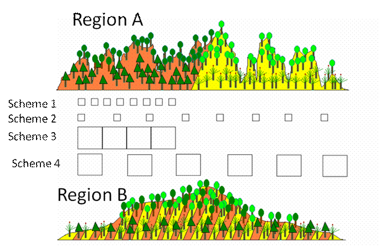
Note that the geometry of the environment differs between regions. Region A has high fine-scale variation in elevation, but only broad-scale variation in bedrock. Region B is the opposite. Nevertheless, the species react to the environment identically in the two regions.

Sampling scheme 1 has both a small grain and a small extent. In region A, such a scheme is likely to reveal an elevation gradient but not a bedrock effect. In region B, it may reveal both.

Sampling scheme 2 has a small grain but large extent. It is likely to reveal both gradients in both sites,

Sampling scheme 3 has a large grain and low extent. In Region A, we might not be able to detect either gradient – the elevational gradient because it is too heterogeneous within the plot, and the bedrock gradient because the extent is small. In Region B, we will not be able to detect the bedrock gradient because it varies within a plot.

Sampling scheme 4, with a large grain and a large extent, is likely to uncover the variables that vary on a broad scale (bedrock in Region A, elevation in Region B), but will be unable to detect the finer-scale patterns because of internal heterogeneity.

Why isn’t sampling scheme 2 always to be preferred, since it seems to be able to reveal patterns of many geometries? It turns out that there are unique problems with small plots. In particular, small plots are likely to capture few individuals, and hence there is more intrinsic variation in composition. You also increase the likelihood of empty plots, which by definition have no species composition whatsoever. In small quadrats, the number of species is so closely tied to the number of individuals or clones sampled (i.e. the ‘rarefaction effect’) and is thus unlikely to be a useful measure for biodiversity studies.

Experimental design for manipulative reserach

Much has been written on the design of manipulative experiments, so I will only briefly treat this topic here.

Randomization

It is important to note that randomization of treatment is just as important as randomization of plot locations. However, you do have a bit of luxury here: you can subjectively select your initial sites (perhaps based on perceived homogeneity, or how closely different sites match each other), as long as this selection is done prior to random selection of the treatments.

Blocks

Very often, we wish to duplicate our experiment in different locations. A simple example might be a greenhouse experiment conducted on different greenhouse benches, because the research will not fit on a single bench. Alternatively, repeating an experiment in different regions will increase the generality of the results. Or perhaps there is known underlying environmental heterogeneity that is not of interest, so we carefully balance the experiment in different environments so we can account for their influence.

Such different locations are known as blocks, and it is often very powerful to use methods that factor out block effects.

Split plot design

One extreme form of block effect is when there is precisely one replicate per treatment in each block. We call this a split plot design.

A split plot design is potentially a very strong design even if you do not consciously stratify by benches, regions, habitats etc. (as in the following example of one treatment and one control) – as it can control for unseen and unknown gradients.

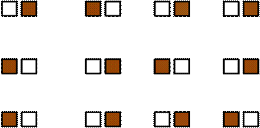
Latin Square

If a balanced design is arranged on a square grid, it is desirable to minimize effects of spatial dependence by having each row and column containing precisely the same number of each treatment . We call such a design a Latin Square. Note that a correctly completed Sudoku puzzle can be considered a special case of a Latin Square..

BACI

Sampling through time is wrought with as much difficulty as sampling through space! For example, we are often interested in trend through time, but temporal dependence (the tendency for something to change more over longer time intervals than shorter time intervals) can lead to incorrect inference. Fortunately, there are methods to correct for temporal trends, though they are not always easy.

It is STRONGLY recommended, whenever possible, to collect data before treatments are imposed. This allows you to evaluate changes through time induced by the treatment, relative to the background changes through time. If proper data are collected, we have a BACI design (for Before-After-Controlled-Impact) and we can use powerful techniques such as principal response curves.

Miscellaneous Advice

Here, I describe some general advice for taking data. We tend to write data sheets in the comfort of an office, forgetting that we are likely use the sheets while being eaten alive by mosquitoes, guarding against sheets blowing away, covered with mud or sweat, suffering from heat or cold, etc. Tiny things that maximize efficiency and comfort will end up paying off in the long run.

Unless you work in a shaded location, the brightness of data sheets can cause serious eyestrain. Print your data sheets on colored paper.

Depending on your climate, print extra data sheets on write-in-the-rain paper.

Most communities contain a few common species and many rare species. Pre-filling your data sheet with common species can help speed collection of data.

To minimize transcription errors and to save time, make the format of your data sheet as close to the format of your spreadsheet or database as possible.

A lot of time (and risk of data loss) in the field occurs when switching data sheets. Try to maximize the amount of data per sheet as long as it does not sacrifice legibility.

If one person takes the data that another person calls out, the latter should proof the data every time to check for legibility and to correct misunderstandings before it is too late to fix.

If it is a new study, only print a few data sheets at a time, and be prepared to revise them. Try to keep track of problems in the field, and what ends up taking more time than necessary. Figure out whether a simple check box may suffice instead of writing out text.

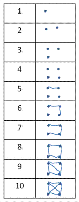
Sometimes we need to take tallies in the field. Most of us are taught to use this kind of tally mark:

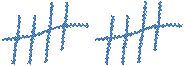
However, this kind (illustrating the numbers 1 through 10) saves space and is easier to use in the long run:

A lot of the advice given in this web page may seem dogmatic or harsh. We should definitely strive towards methodological purity, but I think we all realize that we often must make compromises, and even very good experiments fall short of being perfect.