Ordination Methods - an overview
Michael W. Palmer
This document presents things in a slightly different way than the rest of the web page, so it might help reiterate the principles presented there.
NOTE: as I originally intended this document for the printed page, I have followed the convention of placing the figures at the end. If you find this distracting, let me know! I can try to reformat it accordingly.
Quantitative community ecology is one of the most challenging branches of modern environmetrics. Community ecologists typically need to analyze the effects of multiple environmental factors on dozens (if not hundreds) of species simultaneously, and statistical errors (both measurement and structural) tend to be huge and ill behaved. It is not surprising, therefore, that ecologists have employed a variety of multivariate approaches for community data. These approaches have been both endogenous and borrowed from other disciplines. The majority of techniques fall into two main groups: classification and ordination. Classification is the placement of species and/or sample units into groups, and ordination is the arrangement or ‘ordering’ of species and/or sample units along gradients. In this chapter, I will describe the use and properties of the most widely used ordination methods.
Although community ecology is a fairly young science, the application of quantitative methods began fairly early (McIntosh 1985). In 1930, Ramensky began to use informal ordination techniques for vegetation. Such informal and largely subjective methods became widespread in the early 1950’s (Whittaker 1967). In 1951, Curtis and McIntosh 1951 developed the ‘continuum index’, which later lead to conceptual links between species responses to gradients and multivariate methods. Shortly thereafter, Goodall (1954) introduced the term ‘ordination’ in an ecological context for Principal Components Analysis. Bray and Curtis (1957) developed polar ordination, which became the first widely-used ordination technique in ecology. Austin (1968) used canonical correlation to assess plant-environment relationships in what may have been the first example of multivariate direct gradient analysis in ecology. In 1973, Hill introduced correspondence analysis, a technique originating in the 1930’s, to ecologists. Correspondence analysis gradually supplanted polar ordination, which today has few practitioners. Fasham (1977) and Prentice (1977) independently discovered and demonstrated the utility of Kruskal’s (1964) nonmetric multidimensional scaling, originally intended as a psychometric technique, for community ecology. Hill (1979) corrected some of the flaws of Correspondence Analysis and thereby created Detrended Correspondence Analysis, which is the most widely used indirect gradient analysis technique today. The software to implement Detrended Correspondence Analysis, DECORANA, became the backbone of many later software packages. Gauch’s (1982) book "Multivariate Analysis in Community Ecology" described ordination in non-technical terms to the average practitioner, and allowed ordination techniques to enter the mainstream. Fuzzy set theory, introduced to ecologists by Roberts (1986), is a promising approach with ties to polar ordination, but has yet to gain many adherents. Ter Braak (1986) ushered in the biggest modern revolution in ordination methods with Canonical Correspondence Analysis. This technique coupled Correspondence Analysis with regression methodologies, and provides for hypothesis testing. Ter Braak and Prentice (1988) developed a theoretical unification of ordination techniques, hence placing gradient analysis on a firm theoretical foundation.
Theory
and background
Ordination methods are essentially operations on a community data matrix (or species by sample matrix). A community data matrix has taxa (usually species) as rows and samples as columns (Table 1) or vice versa. In community ecology, the term "sample" has diverged from its usage in statistics, and refers to the basic unit of observation. In most studies of vegetation, the sample is a quadrat, relevé, or transect – though it may consist of a number of subsamples (as is the case with Table 1). Samples in animal ecology may consist of traps, seine sweeps, or survey routes. Biogeographic studies may rely on the cells of large grids or political units as samples.
The elements in community data matrices are abundances of the species. ‘Abundance’ is a general term that can refer to density, biomass, cover, or even incidence (presence/absence) of species. The choice of an abundance measure will depend on the taxa and the questions under consideration. Any of the matrix’s constituent column vectors is considered the species composition for the corresponding sample. Species composition is frequently expressed in terms of relative abundance; i.e. constrained to a constant total such as 1 or 100%. The purpose of ordination and classification methods is to interpret patterns in species composition.
Regardless of the scale or taxa involved, most community data matrices share some general properties:
· They tend to be sparse: a large portion (often the majority) of entries consists of zeros.
· Most species are infrequent. That is, the majority of species is typically present in a minority of locations, and contributes little to the overall abundance.
· The number of factors influencing species composition is potentially very large. For example, forest tree density can be influenced by time since fire, elevation, nutrients, soil depth, soil texture, water availability and many other factors.
· The number of important factors is typically few. That is, a few factors can explain the majority of the explainable variation. Another way of saying this is that the intrinsic dimensionality is low.
· There is much noise. Even under ideal circumstances, replicate samples will vary substantially from each other. This is largely due to stochastic events and contingency (sensu Parker and Peterson 1998), though observer error may also be appreciable.
· There is much redundant information: species often share similar distributions. For example, the abundance of Haplohymenium triste gives some insights into the abundance of Anomodon rostratus, and the abundance of Dicranum montanum helps predict the abundance of Leucobryum albidum (Table 1). It is this property of redundancy that allows us to make sense of compositional data.
For any ordination method to be generally useful, it must be able to cope with the above properties of community data matrices.
Coenospace
As mentioned in the introduction, ordination is the arrangement of species and/or samples along gradients. Indeed, ordination can be considered a synonym for multivariate gradient analysis. Therefore, before discussing ordination, it is necessary to describe an underlying model of species responses to gradients. Although ecologists had a basic understanding environmental control of species composition since the beginning of ecology (McIntosh 1985), Whittaker (1967, 1969) provided a formalization of terms and concepts for the unimodal model. Simply put, the unimodal modal states that species response functions (i.e. the relationship between the abundance of species as a function of position along a gradient) are unimodal, or one-peaked (Figure 1). In other words, there is a unique set of optimal conditions for a species, at which the species has maximal abundance. As conditions differ from this optimum, to the extent of the difference, abundance will decrease. Although Figure1 displays the response of a species to a single gradient, the unimodal modal is readily extended to multiple gradients.
A coenocline is a pictorial representation of all species response functions combined along a single gradient (Figure 2). Given the large number of species and the high noise in most studies, coenoclines are usually only displayed in highly simplified form. Nevertheless, they are useful heuristic concepts. Coenoplanes (2 environmental gradients) and coenospaces (>2 gradients) are even more difficult to display. However, an ordination biplot (discussed later) is an abstracted depiction of coenospace.
Although there are occasionally exceptions to the unimodal model (e.g. bimodal distributions, or qualitative noise due to vicariance events), the model is reasonable for most ecological systems. However, refining the model by assigning functional forms to species response functions has proven difficult (Austin 1987). Gaussian functions (or Gaussian logit functions; ter Braak and Looman 1987) are attractive because they are controlled by relatively few parameters. In addition, a Gaussian assumption leads to elegant proofs and simplifications (ter Braak and Looman 1986). However, other functions (e.g. the Beta function, Minchin 1987) are needed to allow skewed, platykurtic, and leptokurtic forms. The price paid for adopting such models is the larger number of parameters needed. In any case, ecological theory is mute regarding the form of species response functions, and choices have typically been made on empirical grounds.
Whittaker’s
(1967, 1969) tied the unimodal model to levels of diversity, three of which
have become central to community ecology: alpha diversity is the
diversity (either measured in terms of a synthetic diversity index or species
richness) of a community; beta diversity (also known as ‘species
turnover’ or ‘differentiation diversity’)is the rate of change in species
composition from one community to another along gradients; gamma diversity
is the diversity of a region or a landscape (Figure 2).
Gamma diversity can be measured in the same units as alpha diversity.
Ecological
theory does not offer guidelines as to the proper spatial scale for
distinguishing "alpha diversity" from "gamma diversity".
Indeed, these scales are arbitrary and depend upon the objectives of the study
(Palmer and White 1994). In practice, we consider alpha diversity to be the
diversity of the individual sample unit or observation, and gamma diversity to
be the diversity of all sample units combined. Beta diversity then becomes a
measure of how distinct the sampling units are along gradients. A gradient with
high beta diversity is considered a ‘long’ gradient because there is much
change in species composition. Ecologists have proposed a number of beta
diversity indices (e.g. Whittaker 1969, Wilson and Mohler
1983, Oksanen and Tonteri 1995); I will discuss one
of these later in the context of Detrended Correspondence Analysis.
Ecological similarity and distance
We consider two samples with similar species composition to be ecologically similar, and two samples which share few species to be ecologically distant. The concept of ecological distance is akin to beta diversity, but it deviates from it in important respects: samples can be ecologically distant due to noise rather than environmental differences, and ecological distance is not measured along gradients. However, some ordination techniques such as NMDS require measures of ecological distance. Numerous measures of ecological distance (or its complement, ecological similarity) are in use (see Legendre and Legendre 1998). Table 2 is an example of a distance matrix, calculated from the data matrix in Table 1. Note several things:
1) The distance matrix is square and symmetric, i.e. its rows are the same as its columns.
2) The diagonals are zero, meaning that there is no difference between a sample and itself. Because of this and the previous observation, distance matrices are frequently represented as a triangular matrix, ignoring the values above and including the diagonal.
3) Some ecological insights can be derived from the matrix. For example, within a genus (e.g. comparing Quercus alba and Quercus rubra) or species (e.g. comparing Liriodendron tulipifera in two sites) of host trees , epiphytic bryophyte communities are similar (low values), but between genera (e.g. between Quercus and Pinus), communities are dissimilar.
4) All information about particular bryophyte species is lost – so any analyses relying on the distance matrix alone will have limits to its interpretability.
According to Gauch (1982): "Ordination primarily endeavors to represent sample and species relationships as faithfully as possible in a low-dimensional space". But why is this objective desirable? There are a number of answers, but most are derived from the ‘properties of community’ data as described above:
1) It is impossible to visualize multiple dimensions simultaneously. While physicists grumble if space exceeds four dimensions, ecologists typically grapple with dozens of dimensions (species and/or samples).
2) A single multivariate analysis saves time, in contrast to a separate univariate analysis for each species.
3) Ideally and typically, dimensions of this ‘low dimensional space’ will represent important and interpretable environmental gradients.
4) If statistical tests are desired, problems of multiple comparisons are diminished when species composition is studied in its entirety
5) Statistical power is enhanced when species are considered in aggregate, because of redundancy
6) By focusing on ‘important dimensions’, we avoid interpreting (and misinterpreting) noise. Thus, ordination is a ‘noise reduction technique’ (Gauch 1982).
7) We can determine the relative importance of different gradients; this is virtually impossible with univariate techniques.
8) Community patterns may differ from population patterns.
9) Some techniques provide a measure of beta diversity
10) The graphical results from most techniques often lead to ready and intuitive interpretations of species-environment relationships.
Exploratory analysis
and hypothesis testing
Reduction of dimensionality is not the only reason to use ordination. Until recently, the primary goal of ordination was considered "exploratory" (Gauch 1982). It was the job of the ecologist to use his or her knowledge and intuition to collect and interpret data; pure objectivity could potentially interfere with the ability to distinguish important gradients. Ordination was often considered as much an art as a science. With the introduction of CCA, testing statistical hypotheses became routine, and it was possible to go beyond mere "exploratory" analysis. (ter Braak 1985). However, rigorous hypothesis testing requires complete objectivity, which results in repeatability and falsifiability. Thus the two basic motivations for ordination, hypothesis testing and exploratory analysis, can potentially conflict with each other. The two approaches can be reconciled with a cross-validation approach, as discussed later.
Ordination and classification (or clustering) are the two main classes of multivariate methods that community ecologists employ. To some degree, these two approaches are complementary. Classification, or putting samples into (perhaps hierarchical) classes, is often useful when one wishes to assign names to, or to map, ecological communities. However, given the continuous nature of communities (Figure 2), ordination can be considered a more ‘natural’ approach. Classification typically produces disappointing results when samples are arranged continuously along gradients. If samples are clumped along gradients, classes are easier to circumscribe, but the results can become unstable in the presence of samples of intermediate species composition.
Ordination itself can assist with subjective classifications (Peet 1980), and one of the leading classification techniques, TWINSPAN, is a derivative of ordination (Hill 1979). Minimum spanning trees and other graphical techniques can assist in the simultaneous display of ordination and classification results (Digby and Kempton 1987). Fuzzy set theory blurs the distinction between ordination and classification (Roberts 1986).
A classification of ordination
Numerous ordination methods have been put forward, but the most common ones are organized in Table 3. The dichotomy between indirect and direct gradient analysis (Gauch 1982, ter Braak and Prentice 1988), while sometimes blurred in practice, is crucial. Indirect gradient analysis utilizes only the species by sample matrix (e.g. Table 1). If there is any information about the environment, it used after indirect gradient analysis, as an interpretative tool. When we perform an indirect analysis, we are essentially asking the species what the most important gradients are. It is entirely possible that the most important gradients are ones for which we have no external data (e.g. intensity of past disturbance), yet indirect analysis will take advantage of redundancy in the data set and display such gradients.
Direct gradient analysis, in contrast, utilizes external environmental data in addition to the species data. In its simplest form, direct gradient analysis is a regression technique. Direct analysis tells us if species composition is related to our measured variables. Ideally, it will be able to do this even if we did not measure the most important gradients (Palmer 1993). Direct analysis allows us to test the null hypothesis that species composition is unrelated to measured variables. A special case of direct gradient analysis is when our ‘measured variables’ are experimentally imposed treatments.
Table 3 also distinguishes between distance-based techniques (derived from distance matrices such as Table 2) and eigenanalysis-based techniques. This distinction is somewhat arbitrary because Principal Coordinates Analysis can be solved through eigenanalysis, and eigenanalysis-based techniques can usually be described in a 'distance framework' (for example, correspondence analysis can be described in terms of chi-squared distances). Eigenanalysis-based methods are further subdivided into linear models and unimodal models (ter Braak and Prentice 1988), although unimodal models appear to perform well even with linear data (ter Braak and Šmilauer 1998).
The techniques in Table 3 are described below.
Subjective ordering of communities along one or more axes can be heuristically useful. For example, Whittaker (1967) arranged communities on axes of exposure and elevation. Fuhlendorf and Smeins (1997; Figure 5) placed communities in the context of fire frequency and grazing intensity. Likewise, species can be placed along axes of their ecological characteristics (e.g. Grime 1979). Such informal techniques need not be quantitative, but to be effective they do need to communicate relevant concepts.
Polar ordination, Principal Coordinates Analysis, and Nonmetric Multidimensional Scaling differ considerably in their algorithms and properties, yet all rely on a distance matrix as input. Thus, they are all highly sensitive to the choice of the distance metric, and they all ‘hide information’. That is, when ordinating samples, the information about species is collapsed.
Polar ordination (PO; Bray and Curtis 1957) arranges samples between endpoints or ‘poles’ according to the distance matrix. In the earliest versions of PO, these endpoints were the two samples with the highest ecological distance between them, or two samples which are suspected of being at opposite ends of an important gradient (thus introducing a degree of subjectivity).
Using the first of these criteria, and the example in Table 2, we define PT3 and PO2 as endpoints of the first axis. We assign PT3 (endpoint 1) a score of zero, and PO2 (endpoint 2) a score of 76 (its distance of separation from endpoint 1). We arrange the remaining samples along the first axis according to their dissimilarity to PT3 and their similarity to PO2, using
Axis 1 score = (D2 + D12 –D22)/2D (1)
Where D is the distance between the endpoints, D1 is the distance between a sample and the first endpoint, and D2 is the distance between a sample and the second endpoint. Table 4 shows the resulting PO axis scores.
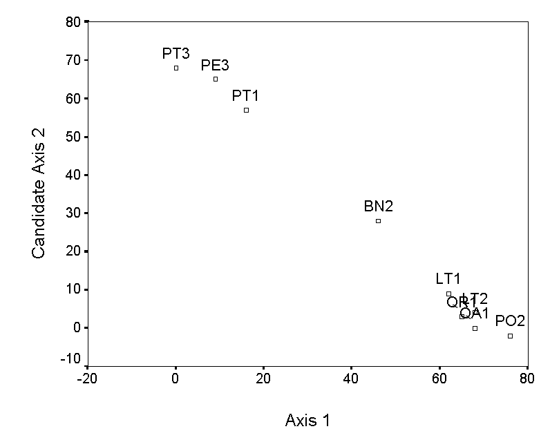
The selection of endpoints for higher axes is a bit more involved. The simplest method is to choose the pair of samples, not including the previous endpoints, with the maximum distance of separation. However, this criterion selects QA1 and PE3, which results in an axis that has a strong negative correlation with axis 1 (Table 4; Figure 3a). This is undesirable, because the second axis contains little information that is not already contained in axis 1. Instead of these endpoints, we choose two samples (QR1 and LT2), which by tedious calculation results in a low correlation with axis 1 (Figure 3b). The ordination diagram is readily interpretable, with the first axis distinguishing bryophyte communities on pine trees from communities on other trees, and the second axis distinguishing oaks from the other hardwoods. These patterns are consistent with others in the literature (cited and reanalyzed in Palmer 1986).
Beals (1984) extended Bray-Curtis ordination and discussed its variants, and is thus a useful reference.
Interpretation of
ordination scatter plots
At this point, it is worth making several observations concerning the interpretation of ordination diagrams (not just from PO):
1) The direction of the axes (e.g. left vs. right; up vs. down) is arbitrary and should not affect the interpretation.
2) The numeric scale on the axis is not very useful for the interpretation (an exception for this is DCA, in which the scales are in units of beta diversity).
3) In PO and most other techniques (but not NMDS), the order of the axes is important. Thus, axis 1 is more important than axis 2, etc. The meaning of ‘importance’ depends on the technique employed, but ideally related to the relative influence of environmental gradients.
4) Third and higher axes can be constructed. The choice of ‘when to stop’ interpreting new axes is largely a matter of taste, the quantity and quality of the data, and the ability to interpret the results. Fortunately, most of the techniques presented later provide supplemental statistics that can assist in the task.
5) It is desirable that axes not be correlated, because you would like them to represent different gradients. Most techniques automatically result in uncorrelated (or orthogonal) axes.
6) A biologist’s insight, experience, and knowledge of the literature are the most important tools for interpreting indirect gradient analysis.
Principal coordinates analysis
Principal coordinates analysis (PCoA) is similar to PO in that it attempts to represent the distances between samples. In particular, it maximizes the linear correlation between the distances in the distance matrix, and the distances in a space of low dimension (typically, 2 or 3 axes are selected). PCoA is perhaps best understood geometrically. The distance between two items can be faithfully represented by one dimension (a line). The distances between three items are faithfully represented by 2 dimensions (a plane): that is, the items will form the vertices of a triangle, a planar object. Distances between four objects define a tetrahedron (a 3-dimensional object). To generalize, distances between N objects can be faithfully represented in N-1 dimensions. Unfortunately, it is difficult for the human mind to grasp more than 3 dimensions simultaneously, so we need to project such multidimensional objects onto lower dimensional space (Figure 4). The PCoA algorithm is analogous to rotating the multidimensional object such that the distances (lines) in the ‘shadow’ are maximally correlated with the distances (connections) in the object.
Although PCoA is based on a distance matrix, the solution can be found by eigenanalysis. When the distance metric is Euclidean, PCoA is equivalent to Principal Components Analysis (thus the bryophyte analysis for PCoA will not be presented here, but rather in the PCA section).
Nonmetric Multidimensional
Scaling
PCoA suffers from a number of flaws, in particular the arch effect (discussed later in the context of PCA and CA). These flaws stem, in part, from the fact that PCoA maximizes a linear correlation. Nonmetric Multidimensional Scaling (NMDS) rectifies this by maximizing the rank order correlation. The algorithm in brief outline, proceeds as follows:
1) The user selects the number of dimensions (N) for the solution, and chooses an appropriate distance metric.
2) The distance matrix is calculated.
3) An initial configuration of samples in N dimensions is selected. This configuration can be random, though the chances of reaching the correct solution are enhanced if the configuration is derived from another ordination method.
4) A measure of ‘stress’ (mismatch between the rank order of distances in the data, and the rank order of distances in the ordination) is calculated
5) The samples are moved slightly in a direction that decreases the stress
6) 4 and 5 are repeated until ‘stress’ appears to reach a minimum. The final configuration of points may be rotated if desired.
The final configuration of points represents your ordination solution. The configuration is dependent on the number of dimensions selected; e.g. the first two axes of a 3-dimensional solution does not necessarily resemble a 2-dimensional solution. The stress will typically decrease as a function of the number of dimensions chosen; this function can aid in the selection of the results. For the bryophyte data of Table 2, the stress is 7.565, 0.881, and 0.001 for the 1, 2, and 3-dimensional solutions, respectively. Thus, the huge drop from the first to the second solution implies that a second axis is useful in explaining species composition. The third dimension is not quite as necessary (i.e. the drop in stress is not as dramatic), but since the stress of a 3D solution is negligible, we will adopt it (Figure 5).
Note that the same gradient in bryophyte species composition appears, as in the case of PO (Figure 3), although in NMDS (Figure 5), the gradient from Pinus species to other host species is reflected in Axis 2. However, recall that in NMDS the order of the axes is arbitrary: the first axis is not necessarily more important than the second axis, etc. This is why it is sometimes useful to rotate the solution (such as by the Varimax method) – although there is no theory that states that the final solution will represent a ‘gradient’ Other problems and advantages of NMDS will be discussed later, when comparing it to Detrended Correspondence Analysis.
Eigenanalysis-based indirect
gradient analysis
What
they are
An introduction to eigenanalysis is beyond the scope of this article. However, in the context of ordination there are several points worth making. For eigenanalysis-based methods:
1) An eigenanalysis is performed on a square, symmetric matrix derived from the data matrix (e.g. Table 1).
2) There is a unique solution to the eigenanalysis, no matter the order of data.
3) Each ordination axis is an eigenvector, and is associated with an eigenvalue. The coordinates for the ith sample along a given axis is the ith element of the axis’ eigenvector.
4) Axes are ranked by their eigenvalues. Thus, the first axis has the highest eigenvalue, the second axis has the second highest eigenvalue, etc.
5) Eigenvalues have mathematical meaning that can aid in interpretation. In principal components analysis, eigenvalues are ‘variance extracted’. In methods related to correspondence analysis, eigenvalues are ‘inertia extracted’, or equivalently, correlation coefficients.
6) Axes are orthogonal to each other.
7) There are a potentially large number of axes (usually, the number of samples minus one, or the number of species minus one, whichever is less) so there is no need to specify the dimensionality in advance. However, the number of dimensions worth interpreting is usually very low.
8) Species and samples are ordinated simultaneously, and can hence both be represented on the same ordination diagram (if this is done, it is termed a biplot).
The simplest and oldest eigenanalysis-based method is Principal Components Analysis (PCA). It is used for many purposes, but I will only discuss its applicability as an ordination method here. Geometrically, PCA is a rigid rotation of the original data matrix, and can be defined as a projection of samples onto a new set of axes, such that the maximum variance is projected or "extracted" along the first axis, the maximum variation uncorrelated with axis 1 is projected on the second axis, the maximum variation uncorrelated with the first and second axis is projected on the third axis, etc. Figure 6 illustrates the similarities between PCA and PCoA (Figure 4).
One of the biggest differences between PCA and PCoA is that the variables (i.e. species) representing the original axes are projected as biplot arrows. In the bryophyte communities (Figure 7), these biplot arrows greatly aid in interpretation. The first axis represents a gradient from communities on Pinus (on the right) to hardwood trees (on the left), with Betula (in the middle) being intermediate. The bryophyte species that point to the lower left are those that dominate on Populus and Quercus, those that dominate on Betula point up, and those that dominate on Pinus point to the right (see Table 1).
The eigenvalues represent the variance extracted by each axis, and are often conveniently expressed as a percentage of the sum of all eigenvalues (i.e. total variance). In the bryophyte example, The first four axes explain approximately 73%, 17%, 4%, and 3% of the variance, respectively. Since the first two axes explain (cumulatively) about 90% of the variance, we deem the 2-dimensional solution of Figure 7 adequate.
In most applications of PCA (e.g. as a factor analysis technique), variables are often measured in different units. For example, PCA of taxonomic data may include measures of size, shape, color, age, numbers, and chemical concentrations. For such data, the data must be standardized to zero mean and unit variance (the typical default for most computer programs). For ordination of ecological communities, however, all species are measured in the same units, and data should not be standardized. In matrix algebra terms, most PCAs are eigenanalyses of the correlation matrix, but for ordination they should be PCAs of the covariance matrix.
In contrast to Correspondence Analysis and related methods (see below), species are represented by arrows. This implies that the abundance of the species is continuously increasing in the direction of the arrow, and decreasing in the opposite direction. Thus PCA is a ‘linear method’.
Although the discussion above implies that PCA is distinctly different from PCoA, the two techniques end up being identical, if the distance metric is Euclidean.
Unfortunately, this linear assumption causes PCA to suffer from a serious problem, the horseshoe effect, which makes it unsuitable for most ecological data sets (Gauch 1982). The PCA solution is often distorted into a horseshoe shape (with the toe either up or down) if beta diversity is moderate to high. The horseshoe can appear even if there is an important secondary gradient. In Figure 7 we cannot easily tell whether BN2 is at one end of a secondary gradient, or if its position at the end of axis 2 is merely a distortion. In extreme cases of the horseshoe effect, the gradient extremes are incurved, resulting in great difficulties of interpretation.
Correspondence Analysis (CA) is also known as reciprocal averaging, because one algorithm for finding the solution involves the repeated averaging of sample scores and species scores (citations). Instead of maximizing ‘variance explained’, CA maximizes the correspondence between species scores and sample scores. First Axis species scores and sample scores are assigned such that the weighted correlation between the two is maximized (Table 1b, Figure 8), where the ‘weight’ is the abundance of the species. Table 1b shows the original bryophyte data matrix, but sorted in order of species scores (rows) and sample scores (columns). Note that the structure of Table 1b is more apparent than in an alphabetical sort (Table 1a). The largest abundances fall on the diagonal, with small values and zeros off the diagonal. Indeed, the resorted table becomes a tabular version of a coenocline (Figure 2): most species have, with some noise, a unimodal response to CA axis 1. As with some of the previous ordinations, the first axis is a gradient from hardwoods to pines, with birch being intermediate.
The eigenvalue of the CA axis is equivalent to the correlation coefficient between species scores and sample scores (Gauch 1982, Pielou 1984). For the bryophyte data, the first eigenvalue is 0.805, which is fairly strong (indeed, the strong correlation can be visualized in Figure 8). It is not possible to arrange rows and/or columns in such a way that makes the correlation higher. The second and higher axes also maximize the correlation between species scores and sample scores, but they are constrained to be uncorrelated with (orthogonal to) the previous axes. The 2nd through 4th axes’ eigenvalues are 0.284, 0.162, and 0.141, implying that the first axis is by far the most important.
If species scores are standardized to zero mean and unit variance, the eigenvalues also represent the variance in the sample scores (but not, as is often misunderstood, the variance in species abundance). In the context of CA, we term this variance the inertia of an axis. The sum of all eigenvalues is the total inertia (1.511 for the bryophyte data). Thus the percentage of inertia ‘extracted’ by the first two axes is 100 * (0.805 + 0.284)/1.511 = 72.1%.
Since CA is a unimodal model, species are represented by a point rather than an arrow (Figure 9). This is (under some choices of scaling; see ter Braak and Šmilauer 1998) the weighted average of the samples in which that species occurs. With some simplifying assumptions (ter Braak and Looman 1987), the species score can be considered an estimate of the location of the peak of the species response curve (Figure 1).
The 2nd and higher axes of the CA solution, like those of PCA, can be distorted for data sets of moderate to high beta diversity (Figure 9). The CA distortion is called the arch effect, which is not as serious as the horseshoe effect of PCA because the ends of the gradients are not incurved. Nevertheless, the distortion is prominent enough to seriously impair ecological interpretation.
In addition to the arch, the axis extremes of CA can be compressed. In other words, the spacing of samples along an axis may not affect true differences in species composition. We suspect this is the case for our data (Figures 8, 9) because the hardwood trees and the pine trees form tight clusters at the opposite end of the first axis – much tighter than would be expected on the basis of dissimilarity (Table 2). Gradient compression can be quite blatant in simulated data sets (Figure 11). The problems of gradient compression and the arch effect led to the development of Detrended Correspondence Analysis.
Detrended Correspondence Analysis
Detrended Correspondence Analysis (DCA) eliminates the arch effect by detrending (Hill and Gauch 1982). There are two basic approaches to detrending: by polynomials and by segments (ter Braak and Šmilauer 1998). Detrending by polynomials is the more elegant of the two: a regression is performed in which the second axis is a polynomial function of the first axis, after which the second axis is replaced by the residuals from this regression. Similar procedures are followed for the third and higher axes. Unfortunately, results of detrending by polynomials can be unsatisfactory and hence detrending by segments is preferred. To detrend the second axis by segments, the first axis is divided up into segments, and the samples within each segment are centered to have a zero mean for the second axis (see illustrations in Gauch 1982). The procedure is repeated for different ‘starting points’ of the segments. Although results in some cases are sensitive to the number of segments (Jackson and Somers 1991), the default of 26 segments is usually satisfactory. Detrending of higher axes proceeds by a similar process.
The compression of the ends of the gradients is corrected by nonlinear rescaling. Rescaling shifts sample scores along each axis such that the average width (or ‘tolerance’; Figure 1) is equal to 1. Figure 11 shows not only how the compression of CA disappears, but also how the species tolerances are equalized (without changing sample order). Rescaling has a beneficial consequence: the axes are scaled in units of beta diversity (SD units, or units of species standard deviations). Thus if the underlying gradient is important well known, it is possible to plot the DCA scores as a function of the gradient, and thereby determine whether the species ‘perceive’ the gradient differently than we measure it (Figure 11). Steeper slopes indicate zones of high beta diversity in such graphs.
Note that the shape of the species response curves may change if axes are rescaled (Figure 11). Thus, skewness and kurtosis are largely artifacts of the units of measurement for which we choose to measure the environment. Since such measures are arbitrary with respect to nature, we are usually not too concerned if the Gaussian model (Figure 1) does not work too well.
For the bryophyte example, DCA no longer shows an arch effect (Figure 10). Because of the rescaling, the minimum sample score is zero for each axis. The maximum sample score is 3.9 along the axis, indicating that approximately 4 standard deviations of species response curves fits along the dominant gradient. With a beta-diversity this high, the samples at the left extreme of the gradient share few species with those at the right (confirmed in Table 1b). The first axis species scores correspond with what we know about the biology of the species: for example, Anomodon attenuatus and Anomodon rostratus are restricted to hardwood trees, and Dicranum scoparium and Leucobryum albidum are restricted to pines and birch. The second DCA axis has a beta diversity of 1.2 standard deviation units, reflecting low beta diversity. Thus, the opposite ends of the second axis are rather similar. A tentative interpretation is that the second axis represents a site effect, with forest #1 having lower scores than forest #2. Such an interpretation would not have been possible with the arch effect in CA (Figure 9). Now that the axes are scaled in units of beta diversity, we can interpret the distances separating samples more easily. For example, the three pine samples remain close together in DCA, indicating their similarity is not merely a result of the gradient compression of CA.
DCA and NMDS are the two most popular methods for indirect gradient analysis. The reason they have remained side-by-side for so long is because, in part, they have different strengths and weaknesses. While the choice between the two is not always straightforward, it is worthwhile outlining a few of the key differences (Table 5). Some of the issues are relatively minor: for example, computation time is rarely an important consideration, except for the hugest data sets. Some issues are not entirely resolved: the degree to which noise affects NMDS, and the degree to which NMDS finds local rather than global options still need to be determined (in the case of the bryophyte data, it took several iterations, with different optimization criteria, before the solution in Figure 5 was reached – so blind acceptance of the first solution is not recommended). Since NMDS is a distance-based method, all information about species identities is hidden once the distance matrix is created. For many, this is the biggest disadvantage of NMDS.
Note that the last two entries in Table 5 do not indicate which method has the advantage. This is perhaps the biggest difference between the two methods: DCA is based on an underlying model of species distributions, the unimodal model, while NMDS is not. Thus, DCA is closer to a theory of community ecology. However, NMDS may be a method of choice if species composition is determined by factors other than position along a gradient: For example, the species present on islands may have more to do with vicariance biogeography and chance extinction events than with environmental preferences – and for such a system, NMDS would be a better a priori choice. As De’ath (1999) points out, there are two classes of ordination methods - ‘species composition restoration’ (e.g. NMDS) and ‘gradient analysis’ (e.g. DCA). The choice between the methods should ultimately be governed by this philosophical distinction.
In direct gradient analysis (DGA), species are directly related to measured environmental factors. Although DGA can be as simple as a scatterplot of species abundance as a function of position along a measured gradient, community data typically have many species and multiple gradients. Thus, DGA is best coupled with a dimension-reduction technique, i.e. ordination. Since multivariate DGA results in axes that are constrained to be a function of measured factors, constrained ordination is a synonym of DGA. In the methods described here, sample scores are constrained to be linear combinations of explanatory variables. As in regression, explanatory (environmental) variables can be continuous or nominal. Unlike ordinary least squares regression, significance is assessed with a Monte Carlo Permutation Procedure, and hence does not rely on distributional assumptions of a test statistic.
The two most commonly used constrained ordination techniques are Redundancy Analysis (RDA) and Canonical Correspondence Analysis (CCA). RDA is the constrained form of PCA, and is inappropriate under the unimodal model. CCA is the constrained form of CA, and therefore is preferred for most ecological data sets (since unimodality is common). CCA also is appropriate under a linear model, as long as one is interested in species composition rather than absolute abundances (ter Braak and Šmilauer 1998). Since most of the discussion concerning CCA also relates to RDA, I will discuss the unique features of RDA briefly after the discussion of CCA.
Canonical Correspondence Analysis
Simply put, Canonical Correspondence Analysis is the marriage between CA and multiple regression. Like CCA, CA maximizes the correlation between species scores and sample scores (Figure 8). However, in CCA the sample scores are constrained to be linear combinations of explanatory variables. Because of the ‘constraint’, eigenvalues in CCA will be lower than in CA.
We can also describe the maximization in CCA as finding the best dispersion of species scores (Figures 12, 13). This view of CCA makes its link to unimodal models clear. If a combination of environmental variables is strongly related to species composition, CCA will create an axis from these variables that makes the species response curves (e.g. Figure 1) most distinct. The second and higher axes will also maximize the dispersion (or inertia) of species, subject to the constraints that these higher axes are linear combinations of the explanatory variables, and that they are orthogonal to all previous axis.
There are as many constrained axes as there are explanatory variables. The total ‘explained inertia’ is the sum of the eigenvalues of the constrained axes. The remaining axes are unconstrained, and can be considered ‘residual’. The total inertia in the species data is the sum of eigenvalues of the constrained and the unconstrained axes, and is equivalent to the sum of eigenvalues, or total inertia, of CA. Thus, explained inertia, compared to total inertia, can be used as a measure of how well species composition is explained by the variables. Unfortunately, a strict measure of ‘goodness of fit’ for CCA is elusive, because the arch effect itself has some inertia associated with it – and it is not always clear whether this inertia belongs in the ‘explained’ or ‘unexplained’ portion.
CCA benefits from the advantages of multiple regression, including:
· It is possible that patterns result from the combination of several explanatory variables; these patterns would not be observable if explanatory variables are considered separately.
· Many extensions of multiple regression (e.g. stepwise analysis and partial analysis) also apply to CCA.
· It is possible to test hypotheses (though in CCA, hypothesis testing is based on randomization procedures rather than distributional assumptions).
· Explanatory variables can be of many types (e.g. continuous, ratio scale, nominal) and do not need to meet distributional assumptions.
Of course, as with multiple regression, one needs to be aware of some caveats:
· In observational studies one cannot necessarily infer direct causation.
· The independent effects of highly correlated variables are difficult to disentangle. However, CCA (and regression) can test the null hypothesis that such variables are completely redundant.
· It is possible to ‘overfit’ the data as the number of variables approaches the number of samples (instead of r2=1, the explained inertia will equal the total inertia and the CCA solution equals the CA solution). The solution is no longer 'constrained' by the variables.
· Noise in explanatory variables will have an effect on the predicted values (McCune 1997). This is not usually a serious problem, because we are typically more interested in environmental variables and species than we are with these predicted values (i.e. sample scores).
· The interpretability of the results is directly dependent on the choice and quality of the explanatory variables.
· Although both multiple regression and CCA find the best linear combination of explanatory variables, they are not guaranteed to find the true underlying gradient (which may be related to unmeasured or unmeasurable factors), nor are they guaranteed to explain a large portion of variation in the data. Some ecologists have rejected CCA and other direct gradient analysis techniques because of this, but finding relationships between measured variables and species composition is actually a desirable attribute.
One of the biggest advantages of CCA lies in the intuitive nature of its ordination diagram, or triplot. It is called a triplot because it simultaneously displays three pieces of information: samples as points, species as points, and environmental variables as arrows (or points). Figure 14 is a triplot of a CCA for the forested vegetation of the Tallgrass Prairie Preserve in Osage County, Oklahoma. Certain species (such as Asimina triloba, Quercus muehlenbergii, Fraxinus muehlenbergii, towards the right of the diagram, are found in conditions of high pH and calcium. Three tree species typical of crosstimbers forests (Quercus stellata, Quercus marilandica, and Carya texana) are found on the left. Crosstimbers forests are generally found on relatively acid (i.e. low pH), sandstone-derived soils (Francaviglia 2000). The arrow representing % cover of water points upwards. Not surprisingly, wetland tree species (Cephalanthus occidentalis and Salix nigra) are located towards the top.
In many, if not most, data sets, CCA triplots can get very crowded. Solutions for this include:
· Separate the parts of the triplot into biplots or scatterplots (e.g. plotting the arrows in a different panel of the same figure)
· Rescaling the arrows so that the species and sample scores are more spread out.
· Only plotting the most abundant species (but by all means, keep the rare species in the analysis).
· Omitting sample scores. After all, they are merely linear combinations of the environment. The samples are, in a sense, ‘tools’ for determining species-environment relationships – so their value as scores is limited. However, it is important to view sample scores to ascertain whether there may be outliers, or gaps in the data.
· Some combination of the above. Whatever is chosen, it is best to keep the particular objective of your study in mind.
Noise in the species abundance data set is not much of a problem for CCA (Palmer 1993). However, it has been argued that noise in the environmental data can be a problem (McCune 1997). It is not at all surprising that noise in the predictor variables will cause noise in the sample scores, since the latter are linear combinations of the former. Although I have not yet put it to a rigorous test, it appears that species scores are much less sensitive to noise in the environment than are sample scores.
Environmental variables in CCA
A concern is often expressed about the use of highly correlated variables. Such redundant variables are very common in ecology. For example, soil pH, and calcium are typically highly correlated with each other. As with multiple regression, it is difficult to disentangle the independent effects of such variables (as in Figure 14). However, they represent no major obstacle for graphical display. They are unlikely to affect the position of species and samples much, and the fact that they all end up pointing the same direction immediately makes their intercorrelations obvious. In general, small angles imply high positive correlations between variables, and arrows pointing in opposite directions will be negatively correlated. It is probably obvious that the choice of variables in CCA is crucial for the output. Meaningless variables will produce meaningless results. However, a meaningful variable that is not necessarily related to the most important gradient may still yield meaningful results (Palmer 1993).
There are only as many ‘constrained’ or ‘canonical’ axes as there are independent environmental variables. Thus, if there are only two variables, the CCA solution is 2-dimensional. However, software packages such as CANOCO will present higher axes. These axes represent the ‘residual’ variation. It is possible for the first residual axis to have a higher eigenvalue than the first constrained axis. Residual axes are very useful in exploratory analyses: they can provide you with hints of what important variables might be missing.
If many variables are included in an analysis, much of the inertia becomes ‘explained’. This is an analogous situation to multiple regression: the multiple r2 or ‘variance explained’ increases as a function of the number of variables included. As the number of variables approaches the number of samples, then the ‘explained inertia’ approaches the total inertia, and the CCA solution approaches the CA solution. In other words, the ordination is no longer ‘constrained’ by the variables. It is very likely that the arch effect, which rarely occurs with low numbers of variables, will appear with higher numbers of variables.
In multiple regression, it is typical to include quadratic terms for explanatory variables. For example, if you expect a response variable to reach a maximum at an intermediate value of an explanatory variable, including this explanatory variable AND the square of the explanatory variable may allow a concave-down parabola to provide a reasonable fit. However, quadratic terms are not to be encouraged in CCA. This would be asking for trouble, as it may force an arch effect to appear.
Explanatory variables need not be continuous in CCA. Indeed, dummy variables representing a categorical variable are very useful. A dummy variable takes the value 1 if the sample belongs to that category, and 0 otherwise. Dummy variables are useful if you have discrete experimental treatments, year effects, different bedrock types, or in the case of the bryophyte example (Table 1), host tree species.
As with regression, the outcome of CCA is highly dependent on the scaling of the explanatory variables. Unfortunately, we cannot know a priori what the best transformation of the data will be, and it would be arrogant to assume that our measurement scale is the same scale used by plants and animals. Nevertheless, we must make intelligent guesses. For example, it is likely that plants do not respond to soil chemical concentrations in a linear way. A 10 ppm difference is much more meaningful at low concentrations than it is at high concentrations. A logarithmic transformation (which emphasizes orders of magnitude of difference rather than absolute difference) is therefore likely to be much closer to the ‘truth’ than a linear scale.
Aspect (compass direction of a slope) clearly must be converted before it can be used. 359 degrees is almost the same direction as 2 degrees. Conversion to dummy variables indicating direction (N, S, E, W) or more detailed (NE, N, NW, W, SW, S, SE, E) or even a 16-point scale might be useful. Alternatively, a trigonometric conversion to an exposure index can be valuable.
Any linear transformation of variables (e.g. kilograms to grams, meters to inches, Fahrenheit to Centigrade) will not affect the outcome of CCA whatsoever.
There are many limitations to CCA (some of these were pointed out by McCune 1997). However, most of these limitations are identical to the limitations of multiple regression. Foremost among these limitations is that correlation does not imply causation, and a variable that appears to be strong may merely be related to an unmeasured but ‘true’ gradient. As with any technique, results should be interpreted in light of these limitations.
Hypothesis testing is straightforward with CCA by means of a randomization test (Manly 1992). The observed first eigenvalue, or the sum of all eigenvalues is calculated for the data. Then this value is compared to the corresponding statistic calculated from each of many random permutations of the data. These permutations keep the actual data intact, but randomly associate the environmental data with the species data. If the true statistic is greater than or equal to 95% of the statistics from the permuted data, we can reject the null hypothesis that species are not related to the environment. The first eigenvalue test determines whether the first CCA axis is stronger than random expectation, and the trace statistic (sum of all canonical axes) tests whether there is an overall relationship between species and environment. Both tests usually yield similar results, but exceptions do occur.
As mentioned previously, most of the discussion of CCA pertains to Redundancy Analysis (RDA). However, note that RDA is a linear method. Some of the special properties of RDA include:
- Since it is a linear method, species as well as
environmental variables are represented by arrows. In most cases, it is
best to represent the two sets of arrows in two figures for ease of
display.
- CCA focuses more on species composition, i.e. relative
abundance. Thus, if you have a gradient along which all
species are positively correlated, RDA will detect such a gradient while
CCA will not.
- With RDA, it is possible to use 'species' that are
measured in different units. If so, the data must be centered and
standardized. But in general, as an ordination technique, the
species should not be standardized.
- RDA can useful when gradients are short. In
particular, RDA may be the method of choice in a short-term experimental
study. In such cases, the treatments are the explanatory variables
(and are usually dummy variables). The sample ID or block might be a
covariable in a partial RDA, if one wishes to factor out local
effects.
- 'variance explained' is
actually a variance explained, and not merely inertia. Thus,
variance partitioning, and interpretation of eigenvalues, are more straightforward
than for CCA.
The relatively short space devoted to RDA should not be given as an indication that it is less valuable than, or inferior to, CCA. When gradients are short it MIGHT be superior. However, note that CCA has a linear face and is thus perfectly acceptable for short gradients.
Future plans:
- Partial
ordination
- Stepwise
CCA
- Cross-validation
- Variance
partitioning
- DCCA
- Choice
between linear and unimodal models
- Fuzzy set
ordination
- Alternative
coordinate systems
- Unfolding
- Multiscale
ordination
Austin, M. P. 1968. An ordination study of a chalk grassland community. J. Ecol. 56:739-57
Austin, M. P. 1987. Models for the analysis of species' response to environmental gradients. Vegetatio 69:35-45
Beals, E. W. 1984. Bray-Curtis ordination: an effective strategy for analysis of multivariate ecological data. Adv. Ecol. Res. 14:1-55
Bray, J. R., and J. T. Curtis. 1957. An ordination of the upland forest communities of southern Wisconsin. Ecol. Mon. 27:325-49
Curtis, J. T., and R. P. McIntosh. 1951. An upland forest continuum in the prairie-forest border region of Wisconsin. Ecology 32:476-96
De'ath, G. 1999. Principal curves: a new technique for indirect and direct gradient analysis. Ecology 80:2237-53
Digby, P. G. N., and R. A. Kempton. 1987. Population and Community Biology Series: Multivariate Analysis of Ecological Communities. Chapman and Hall, London.
Fasham, M. J. R. 1977. A comparison of nonmetric multidimensional scaling, principal components and reciprocal averaging for the ordination of simulated coenoclines and coenoplanes. Ecology 58:551-61
Francaviglia, R. V. 2000. The Cast Iron Forest. University of Texas Press, Austin.
Fuhlendorf, S. D., and F. E. Smeins. 1997. Long-term vegetation dynamics mediated by herbivores, weather and fire in a Juniperus-Quercus savanna. J. Veg. Sci. 8:819-28
Gauch, H. G., Jr. 1982. Multivariate Analysis and Community Structure. Cambridge University Press, Cambridge.
Gauch, H. G., Jr. 1982. Noise reduction by eigenvalue ordinations. Ecology 63:1643-9
Goodall, D. W. 1954. Objective methods for the classification of vegetation. III. An essay in the use of factor analysis. Austral. J. Bot. 1:39-63
Grime, J. P. 1979. Plant strategies and vegetation processes. Wiley & Sons, Chichester.
Hill, M. O. 1979. DECORANA - A FORTRAN program for detrended correspondence analysis an reciprocal averaging. Cornell University, Ithaca, New York.
Hill, M. O. 1979. TWINSPAN - A FORTRAN programme for arranging multivariate data in an ordered two-way table by classification of individuals and attributes. Cornell University, Ithaca, New York.
Hill, M. O. 1973. Reciprocal averaging: an eigenvector method of ordination. J. Ecol. 61:237-49
Kruskal, J. B. 1964. Nonmetric multidimensional scaling: a numerical method. Psychometrika 29:115-29
Legendre, P., and L. Legendre. 1998. Numerical Ecology, 2nd English Edition. Elsevier, Amsterdam.
Manly, B. F. J. 1992. Randomization and Monte Carlo methods in biology. Chapman and Hall, New York.
McCune, B. 1997. Influence of noisy environmental data on canonical correspondence analysis. Ecology 78:2617-23
McIntosh, R. P. 1985. The Background of Ecology. Cambridge University Press, Cambridge, Great Britain.
Minchin, P. R. 1987. Simulation of multidimensional community patterns: towards a comprehensive model. Vegetatio 71:145-56
Oksanen, J., and T. Tonteri. 1995. Rate of compositional turnover along gradients and total gradient length. J. Veg. Sci. 6:815-24
Palmer, M. W. 1986. Pattern in corticolous bryophyte communities of the North Carolina piedmont: Do mosses see the forest or the trees? Bryologist 89:59-65
Palmer, M. W. 1993. Putting things in even better order: the advantages of canonical correspondence analysis. Ecology 74:2215-30
Palmer, M. W., and P. S. White. 1994. On the existence of communities. J. Veg. Sci. 5:279-82
Peet, R. K. 1980. Ordination as a tool for analyzing complex data sets. Vegetatio 42:171-4
Pielou, E. C. 1984. The Interpretation of Ecological Data: A Primer on Classification and Ordination. Wiley, New York.
Prentice, I. C. 1977. Non-metric ordination methods in ecology. J. Ecol. 65:85-94
Roberts, D. W. 1986. Ordination on the basis of fuzzy set theory. Vegetatio 66:123-31
ter Braak, C. J. F. 1985. CANOCO - A FORTRAN program for canonical correspondence analysis and detrended correspondence analysis. IWIS-TNO, Wageningen, The Netherlands.
ter Braak, C. J. F. 1986. Canonical correspondence analysis: a new eigenvector technique for multivariate direct gradient analysis. Ecology 67:1167-79
ter Braak, C. J. F., and C. W. N. Looman. 1987. Regression. Pages 29-77 in R. H. G. Jongman, C. J. F. ter Braak and O. F. R. van Tongeren, editors. Data Analysis in Community and Landscape Ecology. Pudoc, Wageningen, The Netherlands.
ter Braak, C. J. F., and C. W. N. Looman. 1986. Weighted averaging, logistic regression and the Gaussian response model. Vegetatio 65:3-11
ter Braak, C. J. F., and I. C. Prentice. 1988. A theory of gradient analysis. Adv. Ecol. Res. 18:271-313
ter Braak, C. J. F., and P. Šmilauer. 1998. CANOCO reference manual and User's guide to Canoco for Windows: Software for Canonical Community Ordination (version 4). Microcomputer Power, Ithaca.
Whittaker, R. H. 1967. Gradient analysis of vegetation. Biol. Rev. 42:207-64
Whittaker, R. H. 1969. Evolution of diversity in plant communities. Brookhaven Symp. Biol. 22:178-95
Wilson, M. V., and C. L. Mohler. 1983. Measuring compositional change along gradients. Vegetatio 54:129-41
Table 1. a) Importance values of bryophyte species (mosses and liverworts) growing on the trunks of trees in three sites within the Duke Forest, North Carolina (Palmer 1986). Importance values are a measure of relative abundance. Each sample represents the average of 10 trees in a given site. A) data sorted alphabetically. B) data with rows and columns sorted in order of Correspondence Analysis species scores and sample scores, respectively. Sample codes indicate the species of tree and the site; BN = Betula nigra, birch; LT = Liriodendron tulipifera, tulip tree; PE = Pinus echinata, shortleaf pine; PO = Platanus occidentalis, sycamore; PT = Pinus taeda, loblolly pine; QR= Quercus rubra, red oak; QA= Quercus alba, white oak. Numbers 1 through 3 equal sites 1 through 3, respectively.
a)
|
Bryophyte species |
BN2 |
LT1 |
LT2 |
PE3 |
PO2 |
PT1 |
PT3 |
QA1 |
QR1 |
|
Amblystegium serpens |
1 |
0 |
5 |
0 |
0 |
0 |
0 |
3.2 |
2.3 |
|
Anomodon attenuatus |
0.9 |
17.6 |
26.4 |
0 |
41.2 |
0 |
0 |
27.3 |
22.4 |
|
Anomodon minor |
2.1 |
1 |
5.4 |
0 |
9.4 |
0 |
0 |
2.4 |
0.6 |
|
Anomodon rostratus |
0 |
0 |
1.4 |
0 |
4.7 |
0 |
0 |
14 |
13.6 |
|
Brachythecium acuminatum |
0 |
3.1 |
0 |
0 |
0 |
0 |
0 |
5.3 |
2.9 |
|
Brachythecium oxycladon |
0.9 |
1.8 |
0.8 |
0 |
1.6 |
0 |
0 |
1.7 |
0.5 |
|
Bryoandersonia illecebra |
1.8 |
3.7 |
2 |
0 |
0.7 |
0 |
0 |
5.9 |
1.6 |
|
Campylium hispidulum |
0.9 |
1.2 |
0 |
0 |
0 |
0 |
0 |
2.2 |
2.6 |
|
Clasmatodon parvulus |
0 |
1 |
8.1 |
0 |
8.3 |
0 |
0 |
1.1 |
0.4 |
|
Dicranum montanum |
1.8 |
0 |
0 |
6.8 |
0 |
5.8 |
9 |
0 |
0 |
|
Dicranum scoparium |
0 |
0 |
0 |
2 |
0 |
7.1 |
0 |
0 |
0 |
|
Entodon seductrix |
0 |
2.8 |
5.4 |
0 |
0.8 |
0 |
0 |
0 |
0 |
|
Frulania eboracensis |
3.7 |
13.1 |
10.1 |
0 |
7 |
0 |
0 |
7.7 |
7.5 |
|
Haplohymenium triste |
0 |
0.6 |
0.6 |
0 |
2.2 |
0 |
0 |
3.8 |
1.3 |
|
Isopterygium tenerum |
16.1 |
4.6 |
2.2 |
30.9 |
1.4 |
26.8 |
18.2 |
0.6 |
2.4 |
|
Leucobryum albidum |
3.1 |
0 |
0 |
44.6 |
0 |
35.9 |
59 |
0 |
0 |
|
Leucodon julaceus |
1.8 |
5.5 |
6.7 |
0 |
6.8 |
0 |
0 |
7.2 |
9.7 |
|
Lophocolea heterophylla |
20.2 |
0.5 |
1.4 |
7.4 |
0 |
8.4 |
0 |
0 |
0.9 |
|
Platygyrium repens |
29.4 |
5.5 |
9.5 |
0 |
2.1 |
3.2 |
0 |
1.8 |
2.3 |
|
Porella platyphylla |
0 |
1.1 |
0.6 |
0 |
0.7 |
0 |
0 |
2.1 |
3.2 |
|
Radula complanata |
0 |
4 |
0 |
0 |
0.9 |
0 |
0 |
2.3 |
6.2 |
|
Radula obconica |
0 |
6.1 |
2.5 |
0 |
3.5 |
0 |
0 |
2.2 |
6.1 |
|
Sematophyllum adnatum |
11 |
7.9 |
6.2 |
6.4 |
3.9 |
7.4 |
6.1 |
4.6 |
5.9 |
|
Thelia asprella |
0 |
3.3 |
0 |
0 |
0 |
0 |
0 |
0.5 |
0.9 |
|
Thuidium delicatulum |
0.9 |
15.6 |
1.6 |
0 |
0.7 |
0 |
0 |
1.5 |
0.4 |
|
Bryophyte species |
QA1 |
PO2 |
QR1 |
LT2 |
LT1 |
BN2 |
PT1 |
PE3 |
PT3 |
CA Axis 1 species scores |
|
Anomodon rostratus |
14 |
4.7 |
13.6 |
1.4 |
0 |
0 |
0 |
0 |
0 |
-0.90 |
|
Haplohymenium triste |
3.8 |
2.2 |
1.3 |
0.6 |
0.6 |
0 |
0 |
0 |
0 |
-0.90 |
|
Brachythecium acuminatum |
5.3 |
0 |
2.9 |
0 |
3.1 |
0 |
0 |
0 |
0 |
-0.86 |
|
Porella platyphylla |
2.1 |
0.7 |
3.2 |
0.6 |
1.1 |
0 |
0 |
0 |
0 |
-0.86 |
|
Anomodon attenuatus |
27.3 |
41.2 |
22.4 |
26.4 |
17.6 |
0.9 |
0 |
0 |
0 |
-0.85 |
|
Clasmatodon parvulus |
1.1 |
8.3 |
0.4 |
8.1 |
1 |
0 |
0 |
0 |
0 |
-0.84 |
|
Radula complanata |
2.3 |
0.9 |
6.2 |
0 |
4 |
0 |
0 |
0 |
0 |
-0.84 |
|
Radula obconica |
2.2 |
3.5 |
6.1 |
2.5 |
6.1 |
0 |
0 |
0 |
0 |
-0.83 |
|
Leucodon julaceus |
7.2 |
6.8 |
9.7 |
6.7 |
5.5 |
1.8 |
0 |
0 |
0 |
-0.80 |
|
Thelia asprella |
0.5 |
0 |
0.9 |
0 |
3.3 |
0 |
0 |
0 |
0 |
-0.78 |
|
Entodon seductrix |
0 |
0.8 |
0 |
5.4 |
2.8 |
0 |
0 |
0 |
0 |
-0.77 |
|
Anomodon minor |
2.4 |
9.4 |
0.6 |
5.4 |
1 |
2.1 |
0 |
0 |
0 |
-0.75 |
|
Frulania eboracensis |
7.7 |
7 |
7.5 |
10.1 |
13.1 |
3.7 |
0 |
0 |
0 |
-0.74 |
|
Amblystegium serpens |
3.2 |
0 |
2.3 |
5 |
0 |
1 |
0 |
0 |
0 |
-0.74 |
|
Bryoandersonia illecebra |
5.9 |
0.7 |
1.6 |
2 |
3.7 |
1.8 |
0 |
0 |
0 |
-0.72 |
|
Thuidium delicatulum |
1.5 |
0.7 |
0.4 |
1.6 |
15.6 |
0.9 |
0 |
0 |
0 |
-0.71 |
|
Campylium hispidulum |
2.2 |
0 |
2.6 |
0 |
1.2 |
0.9 |
0 |
0 |
0 |
-0.71 |
|
Brachythecium oxycladon |
1.7 |
1.6 |
0.5 |
0.8 |
1.8 |
0.9 |
0 |
0 |
0 |
-0.71 |
|
Platygyrium repens |
1.8 |
2.1 |
2.3 |
9.5 |
5.5 |
29.4 |
3.2 |
0 |
0 |
-0.08 |
|
Sematophyllum adnatum |
4.6 |
3.9 |
5.9 |
6.2 |
7.9 |
11 |
7.4 |
6.4 |
6.1 |
0.10 |
|
Lophocolea heterophylla |
0 |
0 |
0.9 |
1.4 |
0.5 |
20.2 |
8.4 |
7.4 |
0 |
0.61 |
|
Isopterygium tenerum |
0.6 |
1.4 |
2.4 |
2.2 |
4.6 |
16.1 |
26.8 |
30.9 |
18.2 |
0.93 |
|
Dicranum scoparium |
0 |
0 |
0 |
0 |
0 |
0 |
7.1 |
2 |
0 |
1.26 |
|
Dicranum montanum |
0 |
0 |
0 |
0 |
0 |
1.8 |
5.8 |
6.8 |
9 |
1.27 |
|
Leucobryum albidum |
0 |
0 |
0 |
0 |
0 |
3.1 |
35.9 |
44.6 |
59 |
1.33 |
|
CA Axis 1 sample scores |
-0.94 |
-0.93 |
-0.86 |
-0.76 |
-0.73 |
0.29 |
1.24 |
1.32 |
1.45 |
Table 2. Euclidean distance matrix for bryophyte communities of the Duke Forest. For abbreviations, see Table 1.
|
BN2 |
LT1 |
LT2 |
PE3 |
PO2 |
PT1 |
PT3 |
QA1 |
QR1 |
|
|
BN2 |
0 |
42 |
43 |
55 |
57 |
46 |
67 |
50 |
46 |
|
LT1 |
42 |
0 |
22 |
61 |
32 |
53 |
68 |
25 |
23 |
|
LT2 |
43 |
22 |
0 |
63 |
19 |
55 |
70 |
20 |
21 |
|
PE3 |
55 |
61 |
63 |
0 |
70 |
11 |
21 |
65 |
62 |
|
PO2 |
57 |
32 |
19 |
70 |
0 |
64 |
76 |
22 |
26 |
|
PT1 |
46 |
53 |
55 |
11 |
64 |
0 |
27 |
58 |
55 |
|
PT3 |
67 |
68 |
70 |
21 |
76 |
27 |
0 |
71 |
69 |
|
QA1 |
50 |
25 |
20 |
65 |
22 |
58 |
71 |
0 |
10 |
|
QR1 |
46 |
23 |
21 |
62 |
26 |
55 |
69 |
10 |
0 |
Table
3. Common
ordination techniques, by category (largely derived from ter Braak and Prentice
1988). The names of the techniques and their acronyms are given in bold. For
further explanation, see text.
Informal
techniques
Indirect gradient
analysis
Distance-based approaches
· Polar ordination, PO (Bray-Curtis ordination)
· Principal Coordinates Analysis, PCoA (Metric multidimensional scaling)
· Nonmetric Multidimensional Scaling, NMDS
Eigenanalysis-based approaches
Linear model
Principal Components Analysis, PCA
Unimodal model
Correspondence Analysis, CA (Reciprocal Averaging)
Detrended Correspondence Analysis, DCA
Direct gradient
analysis
·
Linear model
Redundancy Analysis, RDA
·
Unimodal model
Canonical Correspondence Analysis,
CCA
Detrended Canonical Correspondence
Analysis, DCCA
Table 4. Polar Ordination Axis scores for the bryophyte data.
|
Axis 1 |
First candidate for Axis 2 |
Second candidate for Axis 2 |
|
|
Endpoint 1 |
PT3 |
QA1 |
QR1 |
|
Endpoint 2 |
PO2 |
PE3 |
LT2 |
|
BN2 |
46 |
28 |
18 |
|
LT1 |
62 |
9 |
12 |
|
LT2 |
68 |
4 |
21 |
|
PE3 |
9 |
65 |
7 |
|
PO2 |
76 |
-2 |
17 |
|
PT1 |
16 |
57 |
8 |
|
PT3 |
0 |
68 |
7 |
|
QA1 |
68 |
0 |
3 |
|
QR1 |
65 |
3 |
0 |
|
Correlation with Axis 1 |
1.000 |
-0.9961 |
0.292841 |
Table 5. Some of the major differences between NMDS and DCA. Bold face indicates what can be considered (in most cases) a better characteristic.
|
|
NMDS |
DCA |
|
Computation time |
High |
Low |
|
Distance metric |
Highly sensitive to choice of distance metric |
Do not
need to specify |
|
Simultaneous ordering of species and samples |
No |
Yes |
|
Arch effect |
Rarely occurs
|
Artificially and inelegantly removed |
|
Related to direct gradient analysis methods |
No |
Yes
|
|
Need to pre-specify numbers of dimensions prior to interpretation |
Yes |
No
|
|
Need to specify parameters for number of segments, etc. |
No
|
Yes
|
|
Solution changes depending upon number of axes viewed |
Yes |
No
|
|
Handles samples with high noise levels |
No(?) |
Yes
|
|
Guaranteed to reach the global solution |
No |
Yes |
|
Results in measures of beta diversity |
No |
Yes
|
|
Used in other disciplines (e.g. psychometry) |
Widely
|
No(?) |
|
Axes interpretable as gradients |
No |
Yes |
|
Derived from a model of species response to gradients |
No |
Yes |
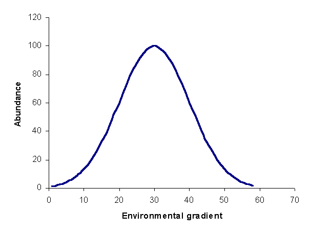
Figure 1: species response curve. For this curve, the optimum is 30, and
the tolerance is 10. Real curves will have much
noise.
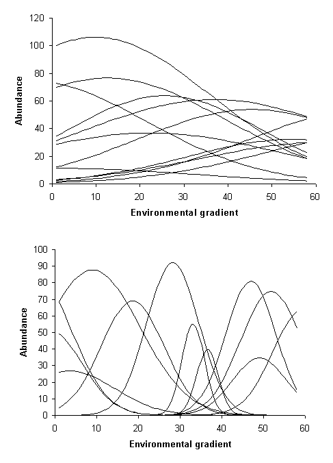
Figure 2: Two coenoclines. Note these are is hypothetical examples;
real examples would have much noise. The top example has lower beta diversity
than the second example.
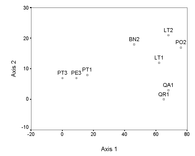
Figure 3. Polar ordination of
the moss example. The second example has a more reasonable second
axis than the first.
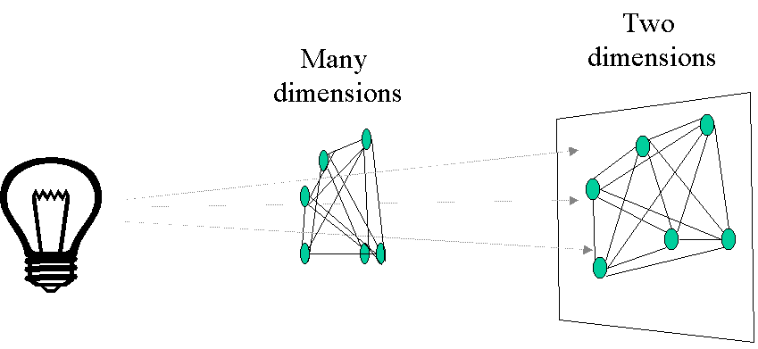
Figure 4.
Principal Coordinates Analysis (PCoA) as a projection
of samples connected by distances.
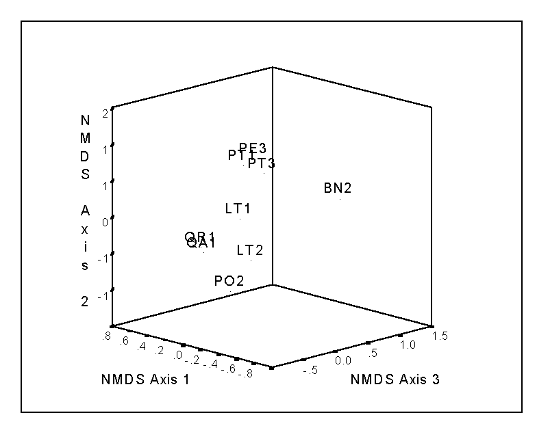
Figure 5.
NMDS of the bryophyte data. Except when there are few
samples, such as with this case, two 2-d plots (e.g. axis 2 vs. axis 1 and axis
3 vs. axis 1) may be better than one 3-d plot.
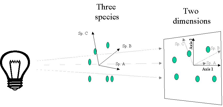
Figure 6.
PCA as a projection of data points. Typical data sets
will have many more than 3 species.
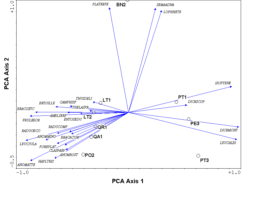
Figure 7.
A PCA biplot of species and samples, produced using
CANOPOST. The species are represented by arrows and the first four
letters of the genus and species name (Table 1)
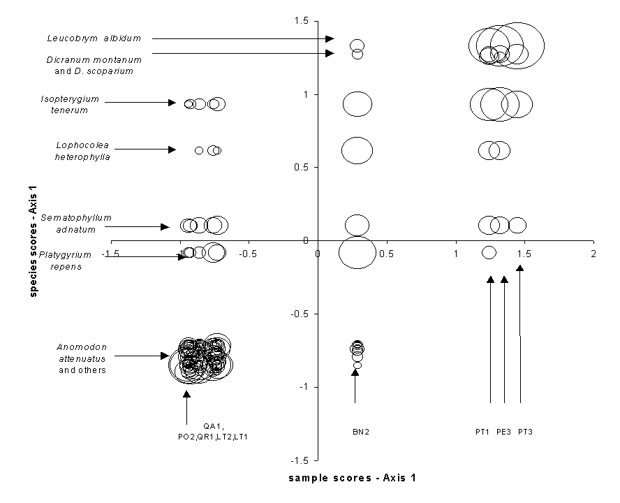
Figure 8.
Correspondence Analysis species scores as a function of sample scores for the
bryophyte data, illustrating the correlation that is maximized between species
and samples.. The sample weight (abundance) is
indicated by the size of the circle.
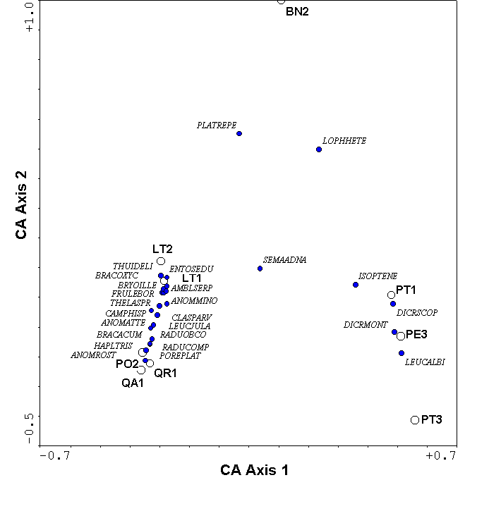
Figure 9.
Correspondence Analysis of the bryophyte data.
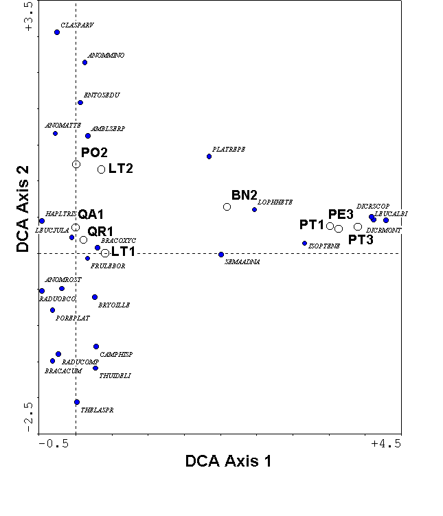
Figure 10.
DCA of the bryophyte data.
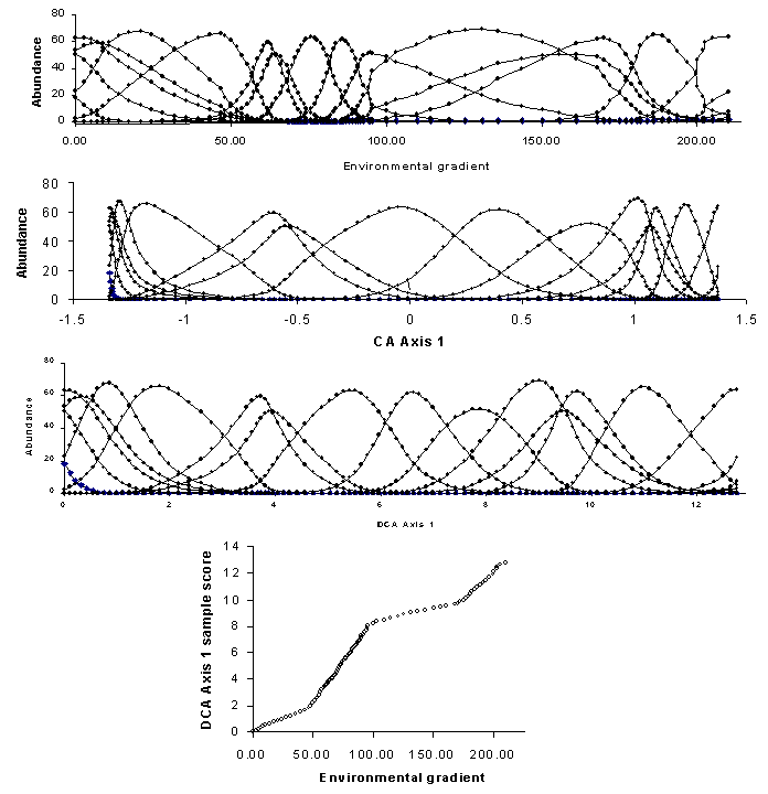
Figure 11: A hypothetical coenocline,
illustrating the compression of CA and the rescaling of DCA.
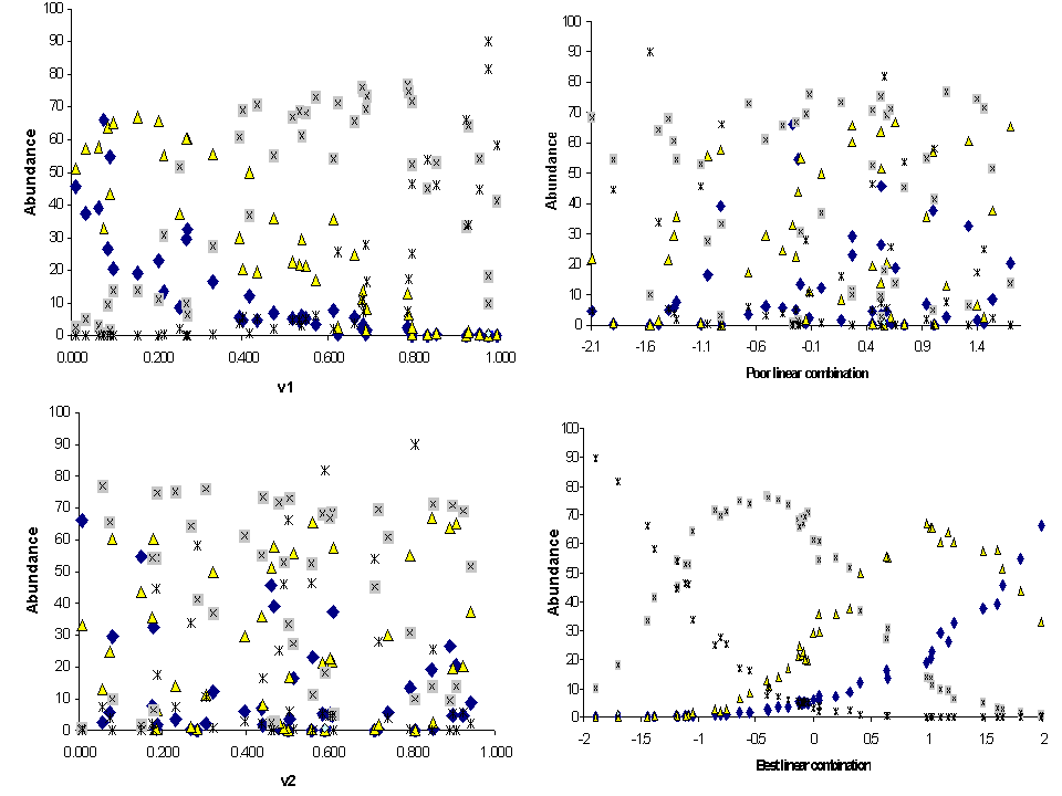
Figure 12. Species abundance as a function of explanatory variables in a
hypothetical 4-species coenocline. Each
species is represented by a different symbol. V1 is a ‘better’ variable than
V2, because species are more clearly segregated along the V1 axis. Species have
no apparent relationship to V2. Species also have no apparent relationships to
the ‘poor’ linear combination (0.1V1 – 0.2V2 + 0.3V3 + 0.7V4) but have very
strong unimodal relationships to the ‘best’ linear combination (-1.0V1 - 0.3V2
+ 0.1V3 - 0.1V4)– which, by definition, is the CCA
first axis. Note that the the ‘best linear combination’
appears to be a cleaned-up version of a mirror image of V1. The mirror image is
because the coefficient for V1 is large and negative.
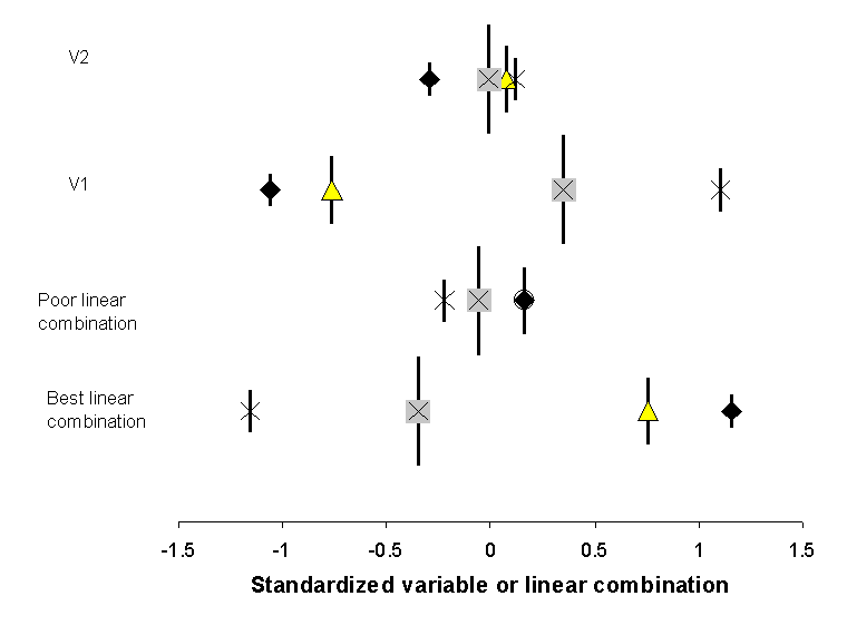
Figure
13. The weighted average location (i.e. species
scores) of the 4 species in Figure 12, as a function
of variables 1, 2, or linear combinations of four explanatory variables.
Symbols for species are the same as in Figure 12, and
vertical bars represent the summed abundance or ‘weight’ of the species. Note
that the spread of scores is greater for V1 than for V2, and better for the
‘best linear combination’ than for the ‘poor linear combination’. CCA chooses
the coefficients for the best linear combination such that the dispersion (or inertia)
of the species scores is maximized.
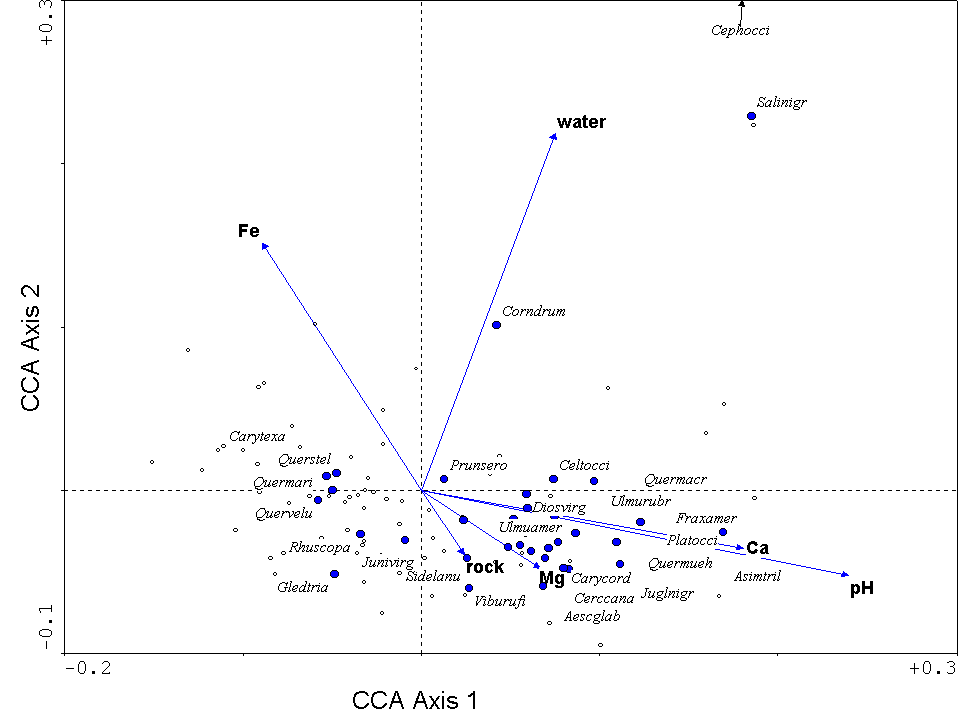
Figure 14. Triplot from a CCA of the forests
in the Tallgrass Prairie Preserve, Oklahoma. Environmental
variables are represented by blue arrows, samples (quadrats) by small open
circles, and species by closed blue circles. The species are listed by
the first four letters of the genus and the specific epithet, they include: Aesculus glabra, Asimina triloba, Carya cordiformis, Carya texana, Celtis occidentalis,
Cephalanthus occidentalis, Cercis canadensis, Cornus drummondii, Diospyros
virginiana, Fraxinus americana, Gleditsia triacanthos, Juglans nigra,
Juniperus virginiana, Platanus occidentalis, Prunus serotina, Quercus macrocarpa, Quercus marilandica, Quercus muehlenbergii,
Quercus stellata, Quercus velutina, Rhus copallina,
Salix nigra, Sideroxylon lanuginosa, Ulmus americana,
Ulmus rubra, Viburnum rufidulum.
