Explorations
in Coenospace
The Data
Matrix
The most common kind of data set in community ecology is the species by sample matrix:
DENSITY OF BIRDS
Species
Sample 1 Sample 2 Sample 3
Cardinals
0
0 0
roadrunners
1
0 0
blue
birds
3
2 0
phoebes
0
0 5
titmice
0
9 6
red-tails
1
0 0
chickadees
20 1
1
waxwings
66
0 0
When we say "data matrix" without any further elaboraton, this is what we usually mean. Samples can be through space or time, or both (that is, it is possible for a given quadrat, sampled on 10 different occasions, to be considered ten samples). Such a data matrix allows us to plot species in sample space, and samples in species space, as well as more complex spaces. See Similarity, Difference, and Distance.
Measures of abundance can include presence/absence, density, biomass, frequency, cover, etc. See Species Abundances in Ordination.
Community data matrices tend to possess the following properties:
- they are sparse (many zeros)
- they have high noise
- they have many rare species (that is, rare in the data
set)
- there are potentially many dimensions
- there are few important dimensions
How
does one make sense of such matrices? By Gradient
Analysis, Classification, and Ordination. Gradient
analysis
- the study of species distributions along gradients.
Direct gradient analysis - gradient analysis in which the important gradients are known and measured. Direct gradient analysis is commonly performed using nonlinear regression (especially using Generalized Linear Modelling), or using a "constrained ordination" technique such as Redundancy Analysis or Canonical Correspondence Analysis.
Indirect gradient analysis - gradients
are unknown a priori,
and
are inferred from species composition data. The species tell us what
the gradients are. This is usually done using an ordination technique such as Detrended Correspondence Analysis.
A graph of the abundance of a species as a function of position along a gradient is called a species response curve.
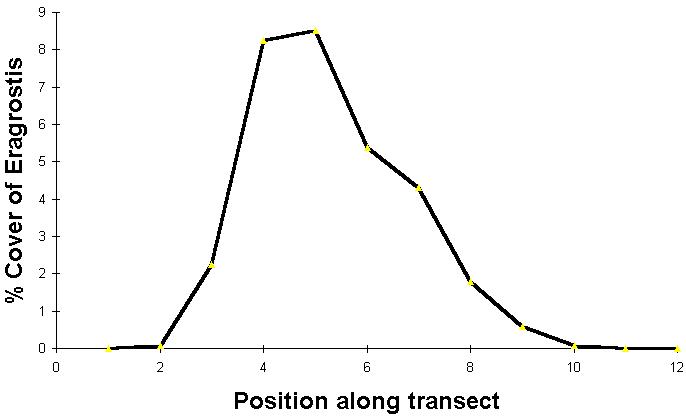
The above example is on the shore of Boomer Lake, a reservoir in Stillwater, Oklahoma. The figure represents the average of 15 transects of 12 contiguous 0.5m x 0.5m plots each. In each transect quadrat #1 is under water, quadrat #2 is just above the water level, and the remaining are increaslingly above the water level.
If long enough gradients are studied, species typically have unimodal (one peak) responses to gradients.
The Gaussian (normal) curve is a reasonable
model, although real curves are seldom truly Gaussian:
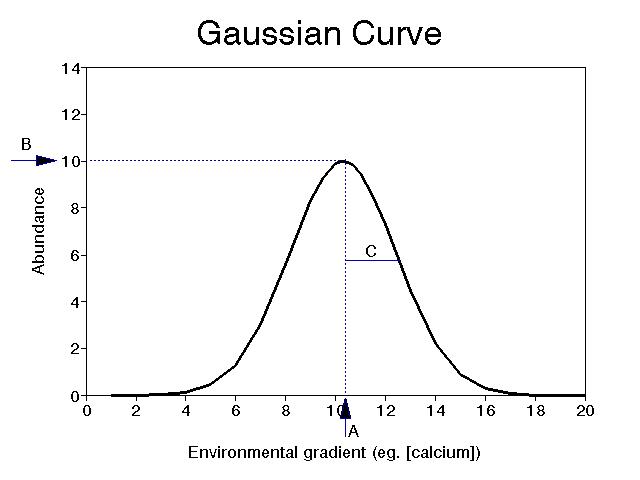
Here, the parameters A, B and C represent the optimum, maximum (or optimal) abundance, and habitat breadth (or species tolerance) respectively.
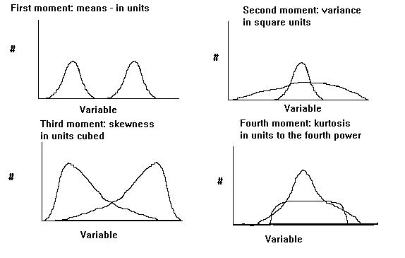
The shape of the species response curve can vary. The optimum is akin to the mean, or the "first moment" of statistics, and the second moment is akin to the variance, or the "second moment" of statistics. Curves which vary in their "higher moments" are not Gaussian anymore. The third moment is related to skewness, or the degree of assymetry, and the fourth moment is related to kurtosis, or "peakedness" of the distribution. One could go on to define even higher moments. However, since part of the purpose of science is to simplify, it is usually best to assume only a few moments, and realize that we can never model nature in all of its complexity.
Coenocline: a figure
representing the distributions of all species
as a function of environmental gradients. (i.e.
all species response curves combined)
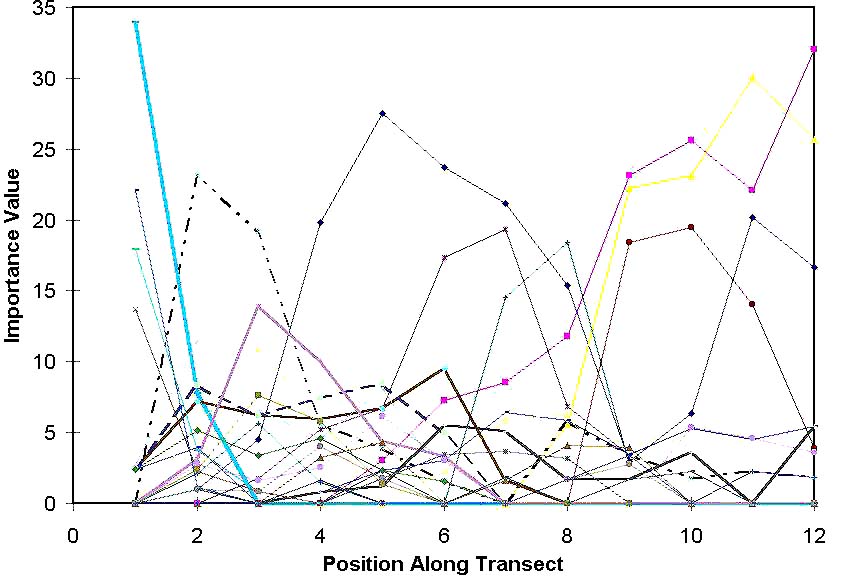
The above is the coenocline for the Boomer Lake study, with all species included.
Coenospace - coenoclines of more than one dimension. These are hard to visualize, but the Multivariate Gaussian Curve is a reasonable model.
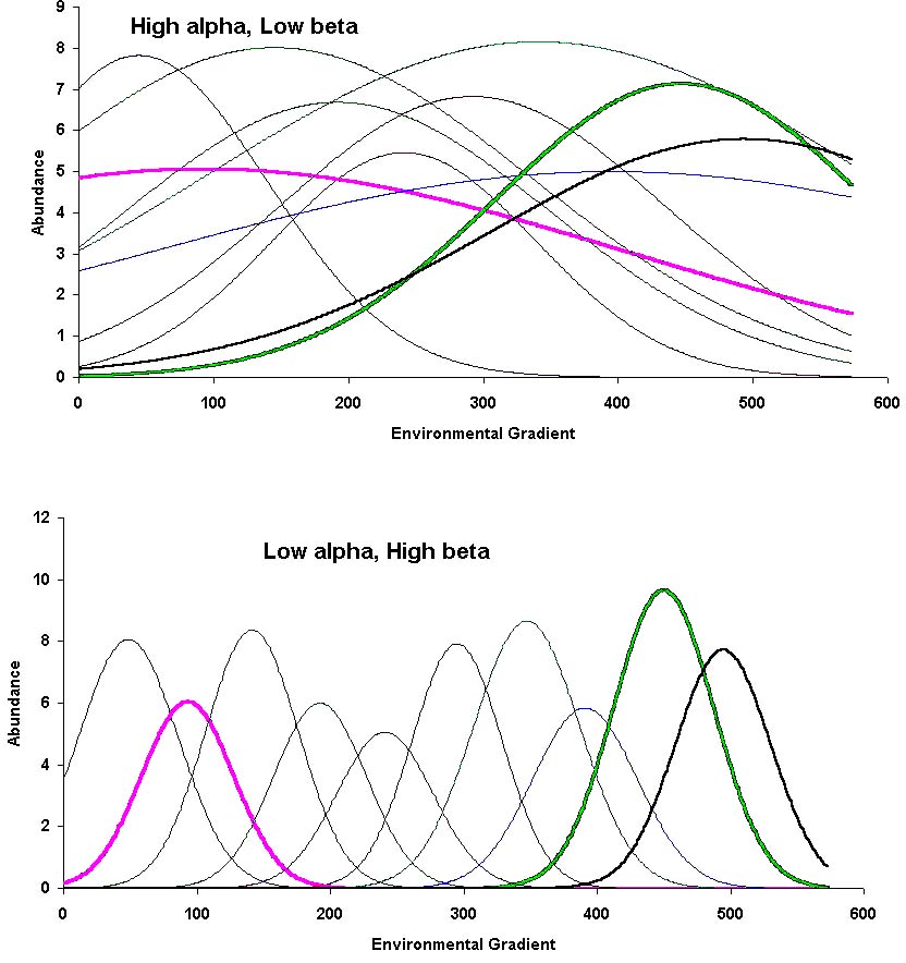
ALPHA,
BETA, AND GAMMA DIVERSITY
alpha diversity: the
diversity of a site
beta diversity: the change in species composition from place to
place, or along environmental gradients
gamma diversity: the diversity of a region or landscape
The following are idealized examples, with no
noise:
Whittaker also described delta and epsilon diversity, which are seldom used today, especially since they are special cases of beta and gamma diversity, respectively.
Alpha and gamma diversity are measured in the same units, e.g. species richness, Shannon index, Simpson index, etc. Beta diversity is fundamentally different. It can be measured in SD units, Gleasons, half-changes, and other indices. (Note: this is a different use of "beta" than we use in the context of regression).
Given an environmental gradient, beta diversity can vary among regions. Also, beta can vary within a gradient. This can be viewed as an artifact - species "see" gradients differently than we do.
The total beta diversity is the "gradient length". A short gradient has low beta diversity.
Total beta can be compared among gradients, but beta diversity not per unit (e.g. one cannot compare whether the rate of change is higher along a pH gradient than along a moisture gradient, but the total change along the gradients can be assessed).
For very short gradients, a unimodal model is not necessary. A simpler, linear model might work.
In the above diagram, only a minority of the species peak within the gradient.
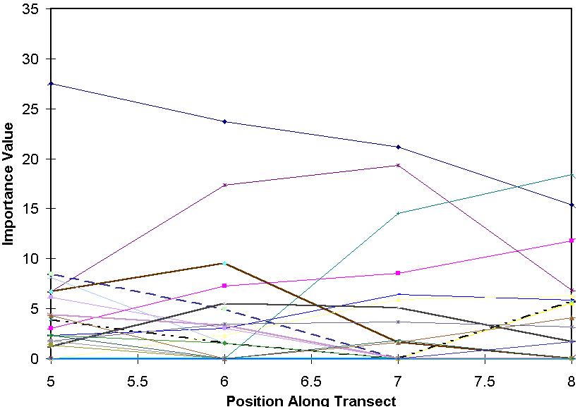
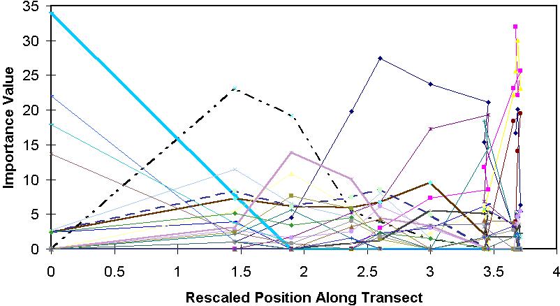
Gradients can be rescaled to constant beta diversity. One way to do this is to stretch and compress parts of the gradient such that the average standard deviation (SD; equivalently the 'tolerance' or 'habitat breadth') of the species response curve is constant. This is what Detrended Correspondence Analysis (DCA) does.
The ability to rescale allows us to convert
skewed curves to symmetrical ones. It can
also allow us to change leptokurtic or platykurtic curves to normal ones. This is why we usually
don't need to care too much if the Gaussian model doesn't work perfectly.
This page was created and is maintained by Michael Palmer.
 To
the ordination web page
To
the ordination web page